Pyleoclim Utilities API (pyleoclim.utils)
Utilities upon which Pyleoclim depends for higher-level functionalities accessible to users.
Pyleoclim makes extensive use of functions from numpy, Pandas, Scipy, Matplotlib, Statsmodels, and scikit-learn. Please note that some default parameter values for these functions have been changed to values more appropriate for paleoclimate datasets.
Causality
Utilities for Liang and Granger causality analysis
- pyleoclim.utils.causality.granger_causality(y1, y2, maxlag=1, addconst=True, verbose=True)[source]
Granger causality tests
Four tests for the Granger non-causality of 2 time series.
All four tests give similar results. params_ftest and ssr_ftest are equivalent based on F test which is identical to lmtest:grangertest in R.
Wrapper for the functions described in statsmodels (https://www.statsmodels.org/stable/generated/statsmodels.tsa.stattools.grangercausalitytests.html)
- Parameters:
y1 (array) – vectors of (real) numbers with identical length, no NaNs allowed
y2 (array) – vectors of (real) numbers with identical length, no NaNs allowed
maxlag (int or int iterable, optional) – If an integer, computes the test for all lags up to maxlag. If an iterable, computes the tests only for the lags in maxlag.
addconst (bool, optional) – Include a constant in the model.
verbose (bool, optional) – Print results
- Returns:
All test results, dictionary keys are the number of lags. For each lag the values are a tuple, with the first element a dictionary with test statistic, pvalues, degrees of freedom, the second element are the OLS estimation results for the restricted model, the unrestricted model and the restriction (contrast) matrix for the parameter f_test.
- Return type:
dict
Notes
The null hypothesis for Granger causality tests is that y2, does NOT Granger cause y1. Granger causality means that past values of y2 have a statistically significant effect on the current value of y1, taking past values of y1 into account as regressors. We reject the null hypothesis that y2 does not Granger cause y1 if the p-values are below a desired threshold (e.g. 0.05).
The null hypothesis for all four test is that the coefficients corresponding to past values of the second time series are zero.
‘params_ftest’, ‘ssr_ftest’ are based on the F distribution
‘ssr_chi2test’, ‘lrtest’ are based on the chi-square distribution
See also
pyleoclim.utils.causality.liang_causalityinformation flow estimated using the Liang algorithm
pyleoclim.utils.causality.signif_isopersistsignificance test with AR(1) with same persistence
pyleoclim.utils.causality.signif_isospecsignificance test with surrogates with randomized phases
References
Granger, C. W. J. (1969). Investigating causal relations by econometric models and cross-spectral methods. Econometrica, 37(3), 424-438.
Granger, C. W. J. (1980). Testing for causality: A personal viewpoont. Journal of Economic Dynamics and Control, 2, 329-352.
Granger, C. W. J. (1988). Some recent development in a concept of causality. Journal of Econometrics, 39(1-2), 199-211.
- pyleoclim.utils.causality.liang(y1, y2, npt=1)[source]
Estimate the Liang information transfer from series y2 to series y1
- Parameters:
y1 (array) – Vectors of (real) numbers with identical length, no NaNs allowed
y2 (array) – Vectors of (real) numbers with identical length, no NaNs allowed
npt (int >=1) – Time advance in performing Euler forward differencing, e.g., 1, 2. Unless the series are generated with a highly chaotic deterministic system, npt=1 should be used
- Returns:
res –
A dictionary of results including:
T21 (float): information flow from y2 to y1 (Note: not y1 -> y2!)
tau21 (float): the standardized information flow from y2 to y1
Z (float): the total information flow from y2 to y1
dH1_star (float): dH*/dt (Liang, 2016)
dH1_noise (float)
- Return type:
dict
See also
pyleoclim.utils.causality.liang_causalityinformation flow estimated using the Liang algorithm
pyleoclim.utils.causality.granger_causalityinformation flow estimated using the Granger algorithm
pyleoclim.utils.causality.signif_isopersistsignificance test with AR(1) with same persistence
pyleoclim.utils.causality.signif_isospecsignificance test with surrogates with randomized phases
References
- Liang, X.S. (2013) The Liang-Kleeman Information Flow: Theory and
Applications. Entropy, 15, 327-360, doi:10.3390/e15010327
- Liang, X.S. (2014) Unraveling the cause-effect relation between timeseries.
Physical review, E 90, 052150
- Liang, X.S. (2015) Normalizing the causality between time series.
Physical review, E 92, 022126
- Liang, X.S. (2016) Information flow and causality as rigorous notions ab initio.
Physical review, E 94, 052201
- pyleoclim.utils.causality.liang_causality(y1, y2, npt=1, signif_test='isospec', nsim=1000, qs=[0.005, 0.025, 0.05, 0.95, 0.975, 0.995])[source]
Liang-Kleeman information flow
Estimate the Liang information transfer from series y2 to series y1 with significance estimates using either an AR(1) tests with series with the same persistence or surrogates with randomized phases.
- Parameters:
y1 (array) – vectors of (real) numbers with identical length, no NaNs allowed
y2 (array) – vectors of (real) numbers with identical length, no NaNs allowed
npt (int >=1) – time advance in performing Euler forward differencing, e.g., 1, 2. Unless the series are generated with a highly chaotic deterministic system, npt=1 should be used
signif_test (str; {'isopersist', 'isospec'}) – the method for significance test see signif_isospec and signif_isopersist for details.
nsim (int) – the number of AR(1) surrogates for significance test
qs (list) – the quantiles for significance test
- Returns:
res – A dictionary of results including: - T21 : float
information flow from y2 to y1 (Note: not y1 -> y2!)
- tau21float
the standardized information flow from y2 to y1
- Zfloat
the total information flow from y2 to y1
- dH1_starfloat
dH*/dt (Liang, 2016)
dH1_noise : float
- signif_qs :
the quantiles for significance test
- T21_noiselist
the quantiles of the information flow from noise2 to noise1 for significance testing
- tau21_noiselist
the quantiles of the standardized information flow from noise2 to noise1 for significance testing
- Return type:
dict
See also
pyleoclim.utils.causality.lianginformation flow estimated using the Liang algorithm
pyleoclim.utils.causality.granger_causalityinformation flow estimated using the Granger algorithm
pyleoclim.utils.causality.signif_isopersistsignificance test with AR(1) with same persistence
pyleoclim.utils.causality.causality.signif_isospecsignificance test with surrogates with randomized phases
References
Liang, X.S. (2013) The Liang-Kleeman Information Flow: Theory and Applications. Entropy, 15, 327-360, doi:10.3390/e15010327
Liang, X.S. (2014) Unraveling the cause-effect relation between timeseries. Physical review, E 90, 052150
Liang, X.S. (2015) Normalizing the causality between time series. Physical review, E 92, 022126
Liang, X.S. (2016) Information flow and causality as rigorous notions ab initio. Physical review, E 94, 052201
- pyleoclim.utils.causality.signif_isopersist(y1, y2, method, nsim=1000, qs=[0.005, 0.025, 0.05, 0.95, 0.975, 0.995], **kwargs)[source]
significance test with AR(1) with same persistence
- Parameters:
y1 (array) – vectors of (real) numbers with identical length, no NaNs allowed
y2 (array) – vectors of (real) numbers with identical length, no NaNs allowed
method (str; {'liang'}) – estimates for the Liang method
nsim (int) – the number of AR(1) surrogates for significance test
qs (list) – the quantiles for significance test
- Returns:
res_dict –
A dictionary with the following information:
T21_noise_qs : list the quantiles of the information flow from noise2 to noise1 for significance testing
tau21_noise_qs : list the quantiles of the standardized information flow from noise2 to noise1 for significance testing
- Return type:
dict
See also
pyleoclim.utils.causality.liang_causalityinformation flow estimated using the Liang algorithm
pyleoclim.utils.causality.granger_causalityinformation flow estimated using the Granger algorithm
pyleoclim.utils.causality.signif_isospecsignificance test with surrogates with randomized phases
- pyleoclim.utils.causality.signif_isospec(y1, y2, method, nsim=1000, qs=[0.005, 0.025, 0.05, 0.95, 0.975, 0.995], **kwargs)[source]
significance test with surrogates with randomized phases
- Parameters:
y1 (array) – vectors of (real) numbers with identical length, no NaNs allowed
y2 (array) – vectors of (real) numbers with identical length, no NaNs allowed
method (str; {'liang'}) – estimates for the Liang method
nsim (int) – the number of surrogates for significance test
qs (list) – the quantiles for significance test
kwargs (dict) – keyword arguments for the causality method (e.g. npt for Liang-Kleeman)
- Returns:
res_dict –
- A dictionary with the following information:
- T21_noise_qslist
the quantiles of the information flow from noise2 to noise1 for significance testing
- tau21_noise_qslist
the quantiles of the standardized information flow from noise2 to noise1 for significance testing
- Return type:
dict
See also
pyleoclim.utils.causality.liang_causalityinformation flow estimated using the Liang algorithm
pyleoclim.utils.causality.granger_causalityinformation flow estimated using the Granger algorithm
pyleoclim.utils.causality.signif_isopersistsignificance test with AR(1) with same persistence
Correlation
Relevant functions for correlation analysis
- pyleoclim.utils.correlation.association(y1, y2, statistic='pearsonr', settings=None)[source]
Quantify the strength of a relationship (e.g. linear) between paired observations y1 and y2.
- Parameters:
y1 (array, length n) – vector of (real) numbers of same length as y2, no NaNs allowed
y2 (array, length n) – vector of (real) numbers of same length as y1, no NaNs allowed
statistic (str, optional) – The statistic used to measure the association, to be chosen from a subset of https://docs.scipy.org/doc/scipy/reference/stats.html#association-correlation-tests [‘pearsonr’,’spearmanr’,’pointbiserialr’,’kendalltau’,’weightedtau’] The default is ‘pearsonr’.
settings (dict, optional) – optional arguments to modify the behavior of the SciPy association functions
- Raises:
ValueError – Complains loudly if the requested statistic is not from the list above.
- Returns:
res – structure containing the result. The first element (res[0]) is always the statistic.
- Return type:
instance result class
- pyleoclim.utils.correlation.corr_ttest(y1, y2, alpha=0.05, df_min=10)[source]
Estimates the significance of correlations between 2 time series using the classical T-test adjusted for effective sample size.
The degrees of freedom are adjusted following n_eff=n(1-g)/(1+g) where g is the lag-1 autocorrelation.
- Parameters:
y1 (array) – vectors of (real) numbers with identical length, no NaNs allowed
y2 (array) – vectors of (real) numbers with identical length, no NaNs allowed
alpha (float) – significance level for critical value estimation [default: 0.05]
df_min (float) – threshold for the effective degrees of freedom, under which things are not computed
- Returns:
r (float) – correlation between x and y
signif (bool) – true (1) if significant; false (0) otherwise
pval (float) – test p-value (the probability of the test statistic exceeding the observed one by chance alone)
See also
pyleoclim.utils.correlation.fdrDetermine significance based on the false discovery rate
- pyleoclim.utils.correlation.cov_shrink_rblw(S, n)[source]
Compute a shrinkage estimate of the covariance matrix using the Rao-Blackwellized Ledoit-Wolf estimator described by Chen et al. 2011 [1]
Contributed by Robert McGibbon.
- Parameters:
S (array, shape=(n, n)) – Sample covariance matrix (e.g. estimated with np.cov(X.T))
n (int) – Number of data points used in the estimate of S.
- Returns:
sigma (array, shape=(p, p)) – Estimated shrunk covariance matrix
shrinkage (float) – The applied covariance shrinkage intensity.
Notes
See the covar documentation for math details.
References
Chen, A. Wiesel and A. O. Hero (2011), Robust Shrinkage Estimation of High-Dimensional Covariance Matrices, IEEE Transactions on Signal Processing, vol. 59, no. 9, pp. 4097-4107, doi:10.1109/TSP.2011.2138698
See also
sklearn.covariance.ledoit_wolfvery similar approach using the same shrinkage target, \(T\), but a different method for estimating the shrinkage intensity, \(gamma\).
- pyleoclim.utils.correlation.fdr(pvals, qlevel=0.05, method='original', adj_method=None, adj_args={})[source]
Determine significance based on the false discovery rate
The false discovery rate is a method of conceptualizing the rate of type I errors in null hypothesis testing when conducting multiple comparisons. Translated from fdr.R by Dr. Chris Paciorek
- Parameters:
pvals (list or array) – A vector of p-values on which to conduct the multiple testing.
qlevel (float) – The proportion of false positives desired.
method ({'original', 'general'}) –
Method for performing the testing.
’original’ follows Benjamini & Hochberg (1995);
’general’ is much more conservative, requiring no assumptions on the p-values (see Benjamini & Yekutieli (2001)).
’original’ is recommended, and if desired, using ‘adj_method=”mean”’ to increase power.
adj_method ({'mean', 'storey', 'two-stage'}) –
Method for increasing the power of the procedure by estimating the proportion of alternative p-values.
’mean’, the modified Storey estimator in Ventura et al. (2004)
’storey’, the method of Storey (2002)
’two-stage’, the iterative approach of Benjamini et al. (2001)
adj_args (dict) – Arguments for adj_method; see prop_alt() for description, but note that for “two-stage”, qlevel and fdr_method are taken from the qlevel and method arguments for fdr()
- Returns:
fdr_res – A vector of the indices of the significant tests; None if no significant tests
- Return type:
array or None
References
fdr.R by Dr. Chris Paciorek: https://www.stat.berkeley.edu/~paciorek/research/code/code.html
- pyleoclim.utils.correlation.fdr_basic(pvals, qlevel=0.05)[source]
The basic FDR of Benjamini & Hochberg (1995).
- Parameters:
pvals (list or array) – A vector of p-values on which to conduct the multiple testing.
qlevel (float) – The proportion of false positives desired.
- Returns:
fdr_res – A vector of the indices of the significant tests; None if no significant tests
- Return type:
array or None
See also
pyleoclim.utils.correlation.fdfDetermine significance based on the false discovery rate
References
Benjamini, Yoav; Hochberg, Yosef (1995). “Controlling the false discovery rate: a practical and powerful approach to multiple testing”. Journal of the Royal Statistical Society, Series B. 57 (1): 289–300. MR 1325392
- pyleoclim.utils.correlation.fdr_master(pvals, qlevel=0.05, method='original')[source]
Perform various versions of the FDR procedure
- Parameters:
pvals (list or array) – A vector of p-values on which to conduct the multiple testing.
qlevel (float) – The proportion of false positives desired.
method ({'original', 'general'}) – Method for performing the testing. - ‘original’ follows Benjamini & Hochberg (1995); - ‘general’ is much more conservative, requiring no assumptions on the p-values (see Benjamini & Yekutieli (2001)). We recommend using ‘original’, and if desired, using ‘adj_method=”mean”’ to increase power.
- Returns:
fdr_res – A vector of the indices of the significant tests; None if no significant tests
- Return type:
array or None
See also
pyleoclim.utils.correlation.fdfDetermine significance based on the false discovery rate
References
Benjamini, Yoav; Hochberg, Yosef (1995). “Controlling the false discovery rate: a practical and powerful approach to multiple testing”. Journal of the Royal Statistical Society, Series B. 57 (1): 289–300. MR 1325392
Benjamini, Yoav; Yekutieli, Daniel (2001). “The control of the false discovery rate in multiple testing under dependency”. Annals of Statistics. 29 (4): 1165–1188. doi:10.1214/aos/1013699998
- pyleoclim.utils.correlation.prop_alt(pvals, adj_method='mean', adj_args={'edf_lower': 0.8, 'num_steps': 20})[source]
Calculate an estimate of a, the proportion of alternative hypotheses, using one of several methods
- Parameters:
pvals (list or array) – A vector of p-values on which to estimate a
- adj_method: str; {‘mean’, ‘storey’, ‘two-stage’}
Method for increasing the power of the procedure by estimating the proportion of alternative p-values. - ‘mean’, the modified Storey estimator that we suggest in Ventura et al. (2004) - ‘storey’, the method of Storey (2002) - ‘two-stage’, the iterative approach of Benjamini et al. (2001)
- adj_argsdict
for “mean”, specify “edf_lower”, the smallest quantile at which to estimate a, and “num_steps”, the number of quantiles to use the approach uses the average of the Storey (2002) estimator for the num_steps quantiles starting at “edf_lower” and finishing just less than 1
for “storey”, specify “edf_quantile”, the quantile at which to calculate the estimator
for “two-stage”, the method uses a standard FDR approach to estimate which p-values are significant this number is the estimate of a; therefore the method requires specification of qlevel, the proportion of false positives and “fdr_method” (‘original’ or ‘general’), the FDR method to be used. We do not recommend ‘general’ as this is very conservative and will underestimate a.
- Returns:
a – estimate of a, the number of alternative hypotheses
- Return type:
int
See also
pyleoclim.utils.correlation.fdfDetermine significance based on the false discovery rate
References
Storey, J.D. (2002). A direct approach to False Discovery Rates. Journal of the Royal Statistical Society, Series B, 64, 3, 479-498
Benjamini, Yoav; Yekutieli, Daniel (2001). “The control of the false discovery rate in multiple testing under dependency”. Annals of Statistics. 29 (4): 1165–1188. doi:10.1214/aos/1013699998
Ventura, V., Paciorek, C., Risbey, J.S. (2004). Controlling the proportion of falsely rejected hypotheses when conducting multiple tests with climatological data. Journal of climate, 17, 4343-4356
- pyleoclim.utils.correlation.storey(edf_quantile, pvals)[source]
The basic Storey (2002) estimator of a, the proportion of alternative hypotheses.
- Parameters:
edf_quantile (float) – The quantile of the empirical distribution function at which to estimate a.
pvals (list or array) – A vector of p-values on which to estimate a
- Returns:
a – estimate of a, the number of alternative hypotheses
- Return type:
int
See also
pyleoclim.utils.correlation.fdfDetermine significance based on the false discovery rate
References
Storey, J.D., 2002, A direct approach to False Discovery Rates. Journal of the Royal Statistical Society, Series B, 64, 3, 479-498
Decomposition
Eigendecomposition methods: Singular Spectrum Analysis (SSA). soon: PCA, Monte-Carlo PCA, Multi-Channel SSA
- pyleoclim.utils.decomposition.ssa(y, M=None, nMC=0, f=0.5, trunc=None, var_thresh=80, online=True)[source]
Singular spectrum analysis
Nonparametric eigendecomposition of timeseries into orthogonal oscillations. This implementation uses the method of [1], with applications presented in [2]. Optionally (nMC>0), the significance of eigenvalues is assessed by Monte-Carlo simulations of an AR(1) model fit to X, using [3]. The method expects regular spacing, but is tolerant to missing values, up to a fraction 0<f<1 (see [4]).
- Parameters:
y (array of length N) – time series (evenly-spaced, possibly with up to f*N NaNs)
M (int) – window size (default: 10% of N)
nMC (int) – Number of iterations in the Monte-Carlo simulation (default nMC=0, bypasses Monte Carlo SSA) Currently only supported for evenly-spaced, gap-free data.
f (float) – maximum allowable fraction of missing values. (Default is 0.5)
trunc (str) –
- if present, truncates the expansion to a level K < M owing to one of 4 criteria:
’kaiser’: variant of the Kaiser-Guttman rule, retaining eigenvalues larger than the median
’mcssa’: Monte-Carlo SSA (use modes above the 95% quantile from an AR(1) process)
’var’: first K modes that explain at least var_thresh % of the variance.
- Default is None, which bypasses truncation (K = M)
’knee’: Wherever the “knee” of the screeplot occurs.
Recommended as a first pass at identifying significant modes as it tends to be more robust than ‘kaiser’ or ‘var’, and faster than ‘mcssa’. While no truncation method is imposed by default, if the goal is to enhance the S/N ratio and reconstruct a smooth version of the attractor’s skeleton, then the knee-finding method is a good compromise between objectivity and efficiency. See kneed’s documentation for more details on the knee finding algorithm.
var_thresh (float) – variance threshold for reconstruction (only impactful if trunc is set to ‘var’)
online (bool; {True,False}) –
Whether or not to conduct knee finding analysis online or offline. Only called when trunc = ‘knee’. Default is True See kneed’s documentation for details.
- Returns:
res –
eigvals : (M, ) array of eigenvalues
eigvecs : (M, M) Matrix of temporal eigenvectors (T-EOFs)
PC : (N - M + 1, M) array of principal components (T-PCs)
RCmat : (N, M) array of reconstructed components
RCseries : (N,) reconstructed series, with mean and variance restored
pctvar: (M, ) array of the fraction of variance (%) associated with each mode
eigvals_q : (M, 2) array containting the 5% and 95% quantiles of the Monte-Carlo eigenvalue spectrum [ if nMC >0 ]
mode_idx : array of indices of eigenvalues >=eigvals_q
- Return type:
dict containing:
References
[1]_ Vautard, R., and M. Ghil (1989), Singular spectrum analysis in nonlinear dynamics, with applications to paleoclimatic time series, Physica D, 35, 395–424.
[2]_ Ghil, M., R. M. Allen, M. D. Dettinger, K. Ide, D. Kondrashov, M. E. Mann, A. Robertson, A. Saunders, Y. Tian, F. Varadi, and P. Yiou (2002), Advanced spectral methods for climatic time series, Rev. Geophys., 40(1), 1003–1052, doi:10.1029/2000RG000092.
[3]_ Allen, M. R., and L. A. Smith (1996), Monte Carlo SSA: Detecting irregular oscillations in the presence of coloured noise, J. Clim., 9, 3373–3404.
[4]_ Schoellhamer, D. H. (2001), Singular spectrum analysis for time series with missing data, Geophysical Research Letters, 28(16), 3187–3190, doi:10.1029/2000GL012698.
See also
pyleoclim.core.series.Series.ssaSingular Spectrum Analysis for timeseries objects
pyleoclim.core.ssares.SsaRes.modeplotplot SSA modes
pyleoclim.core.ssares.SsaRes.screeplotplot SSA eigenvalue spectrum
Filter
Utilities to filter arrayed timeseries data, leveraging SciPy
- pyleoclim.utils.filter.butterworth(ys, fc, fs=1, filter_order=3, pad='reflect', reflect_type='odd', params=(1, 0, 0), padFrac=0.1)[source]
- Applies a Butterworth filter with frequency fc, with padding
Supports both lowpass and band-pass filtering.
- Parameters:
ys (numpy array) – Timeseries
fc (float or list) – cutoff frequency. If scalar, it is interpreted as a low-frequency cutoff (lowpass) If fc is a list, it is interpreted as a frequency band (f1, f2), with f1 < f2 (bandpass)
fs (float) – sampling frequency
filter_order (int) – order n of Butterworth filter
pad (str) –
Indicates if padding is needed.
’reflect’: Reflects the timeseries
’ARIMA’: Uses an ARIMA model for the padding
None: No padding.
params (tuple) – model parameters for ARIMA model (if pad = ‘ARIMA’)
padFrac (float) – fraction of the series to be padded
- Returns:
yf – filtered array
- Return type:
array
See also
pyleoclim.utils.filter.ts_padPad a timeseries based on timeseries model predictions
pyleoclim.utils.filter.firwinApplies a Finite Impulse Response filter with frequency fc, with padding
pyleoclim.utils.filter.savitzky_golaySmooth (and optionally differentiate) data with a Savitzky-Golay filter
pyleoclim.utils.filter.lanczosApplies a Lanczos filter with frequency fc, with padding
- pyleoclim.utils.filter.firwin(ys, fc, numtaps=None, fs=1, pad='reflect', window='hamming', reflect_type='odd', params=(1, 0, 0), padFrac=0.1, **kwargs)[source]
Applies a Finite Impulse Response filter design with window method and frequency fc, with padding
- Parameters:
ys (numpy array) – Timeseries
fc (float or list) – cutoff frequency. If scalar, it is interpreted as a low-frequency cutoff (lowpass) If fc is a list, it is interpreted as a frequency band (f1, f2), with f1 < f2 (bandpass)
numptaps (int) – Length of the filter (number of coefficients, i.e. the filter order + 1). numtaps must be odd if a passband includes the Nyquist frequency. If None, will use the largest number that is smaller than 1/3 of the the data length.
fs (float) – sampling frequency
window (str or tuple of string and parameter values, optional) – Desired window to use. See scipy.signal.get_window for a list of windows and required parameters.
pad (str) –
Indicates if padding is needed.
’reflect’: Reflects the timeseries
’ARIMA’: Uses an ARIMA model for the padding
None: No padding.
params (tuple) – model parameters for ARIMA model (if pad = True)
padFrac (float) – fraction of the series to be padded
kwargs (dict) – a dictionary of keyword arguments for scipy.signal.firwin
- Returns:
yf – filtered array
- Return type:
array
See also
scipy.signal.firwinFIR filter design using the window method. See https://docs.scipy.org/doc/scipy/reference/generated/scipy.signal.get_window.html#scipy.signal.get_window
pyleoclim.utils.filter.ts_padPad a timeseries based on timeseries model predictions
pyleoclim.utils.filter.butterworthApplies a Butterworth filter with frequency fc, with padding
pyleoclim.utils.filter.lanczosApplies a Lanczos filter with frequency fc, with padding
pyleoclim.utils.filter.savitzky_golaySmooth (and optionally differentiate) data with a Savitzky-Golay filter
- pyleoclim.utils.filter.lanczos(ys, fc, fs=1, pad='reflect', reflect_type='odd', params=(1, 0, 0), padFrac=0.1)[source]
Applies a Lanczos (lowpass) filter with frequency fc, with optional padding
- Parameters:
ys (numpy array) – Timeseries
fc (float) – cutoff frequency
fs (float) – sampling frequency
pad (str) –
Indicates if padding is needed
’reflect’: Reflects the timeseries
’ARIMA’: Uses an ARIMA model for the padding
None: No padding
params (tuple) – model parameters for ARIMA model (if pad = ‘ARIMA’). May require fiddling
padFrac (float) – fraction of the series to be padded
- Returns:
yf – filtered array
- Return type:
array
See also
pyleoclim.utils.filter.ts_padPad a timeseries based on timeseries model predictions
pyleoclim.utils.filter.butterworthApplies a Butterworth filter with frequency fc, with padding
pyleoclim.utils.filter.firwinApplies a Finite Impulse Response filter with frequency fc, with padding
pyleoclim.utils.filter.savitzky_golaySmooth (and optionally differentiate) data with a Savitzky-Golay filter
References
Filter design from http://scitools.org.uk/iris/docs/v1.2/examples/graphics/SOI_filtering.html
- pyleoclim.utils.filter.savitzky_golay(ys, window_length=None, polyorder=2, deriv=0, delta=1, axis=-1, mode='mirror', cval=0)[source]
Smooth (and optionally differentiate) data with a Savitzky-Golay filter.
The Savitzky-Golay filter removes high frequency noise from data. It has the advantage of preserving the original shape and features of the signal better than other types of filtering approaches, such as moving averages techniques.
The Savitzky-Golay is a type of low-pass filter, particularly suited for smoothing noisy data. The main idea behind this approach is to make for each point a least-square fit with a polynomial of high order over a odd-sized window centered at the point.
Uses the implementation from scipy.signal: https://docs.scipy.org/doc/scipy/reference/generated/scipy.signal.savgol_filter.html
- Parameters:
ys (array) – the values of the signal to be filtered
window_length (int) – The length of the filter window. Must be a positive integer. If mode is ‘interp’, window_length must be less than or equal to the size of ys. Default is the size of ys.
polyorder (int) – The order of the polynomial used to fit the samples. polyorder Must be less than window_length. Default is 2
deriv (int) – The order of the derivative to compute. This must be a nonnegative integer. The default is 0, which means to filter the data without differentiating
delta (float) – The spacing of the samples to which the filter will be applied. This is only used if deriv>0. Default is 1.0
axis (int) – The axis of the array ys along which the filter will be applied. Default is -1
mode (str) – Must be ‘mirror’ (the default), ‘constant’, ‘nearest’, ‘wrap’ or ‘interp’. This determines the type of extension to use for the padded signal to which the filter is applied. When mode is ‘constant’, the padding value is given by cval. See the Notes for more details on ‘mirror’, ‘constant’, ‘wrap’, and ‘nearest’. When the ‘interp’ mode is selected, no extension is used. Instead, a degree polyorder polynomial is fit to the last window_length values of the edges, and this polynomial is used to evaluate the last window_length // 2 output values.
cval (scalar) – Value to fill past the edges of the input if mode is ‘constant’. Default is 0.0.
- Returns:
yf – ndarray of shape (N), the smoothed signal (or its n-th derivative).
- Return type:
array
See also
pyleoclim.utils.filter.butterworthApplies a Butterworth filter with frequency fc, with padding
pyleoclim.utils.filter.lanczosApplies a Lanczos filter with frequency fc, with padding
pyleoclim.utils.filter.firwinApplies a Finite Impulse Response filter with frequency fc, with padding
References
Savitzky, M. J. E. Golay, Smoothing and Differentiation of Data by Simplified Least Squares Procedures. Analytical Chemistry, 1964, 36 (8), pp 1627-1639.
Numerical Recipes 3rd Edition: The Art of Scientific Computing W.H. Press, S.A. Teukolsky, W.T. Vetterling, B.P. Flannery Cambridge University Press ISBN-13: 9780521880688
Notes
Details on the mode option:
‘mirror’: Repeats the values at the edges in reverse order. The value closest to the edge is not included.
‘nearest’: The extension contains the nearest input value.
‘constant’: The extension contains the value given by the cval argument.
‘wrap’: The extension contains the values from the other end of the array.
- pyleoclim.utils.filter.ts_pad(ys, ts, method='reflect', params=(1, 0, 0), reflect_type='odd', padFrac=0.1)[source]
Pad a timeseries based on timeseries model predictions
- Parameters:
ys (numpy array) – Evenly-spaced timeseries
ts (numpy array) – Time axis
method (str) –
the method to use to pad the series
ARIMA: uses a fitted ARIMA model
reflect (default): Reflects the time series around either end.
params (tuple) – the ARIMA model order parameters (p,d,q), Default corresponds to an AR(1) model
reflect_type (str; {‘even’, ‘odd’}, optional) – Used in ‘reflect’, and ‘symmetric’. The ‘even’ style is the default with an unaltered reflection around the edge value. For the ‘odd’ style, the extented part of the array is created by subtracting the reflected values from two times the edge value. For more details, see np.lib.pad()
padFrac (float) – padding fraction (scalar) such that padLength = padFrac*length(series)
- Returns:
yp (array) – padded timeseries
tp (array) – augmented time axis
See also
pyleoclim.utils.filter.butterworthApplies a Butterworth filter with frequency fc, with padding
pyleoclim.utils.filter.lanczosApplies a Lanczos filter with frequency fc, with padding
pyleoclim.utils.filter.firwinApplies a Finite Impulse Response filter with frequency fc, with padding
Mapping
Mapping utilities for geolocated objects, leveraging Cartopy.
- pyleoclim.utils.mapping.compute_dist(lat_r, lon_r, lat_c, lon_c)[source]
Computes the distance in (km) between a reference point and an array of other coordinates.
- Parameters:
lat_r (float) – The reference latitude, in deg
lon_r (float) – The reference longitude, in deg
lat_c (list) – A list of latitudes for the comparison points, in deg
lon_c (list) – A list of longitudes for the comparison points, in deg
- Returns:
dist – A list of distances in km.
- Return type:
list
See also
pyleoclim.utils.mapping.dist_spherecalculate distance on a sphere
- pyleoclim.utils.mapping.dist_sphere(lat1, lon1, lat2, lon2)[source]
Uses the haversine formula to calculate distance on a sphere https://en.wikipedia.org/wiki/Haversine_formula
- Parameters:
lat1 (float) – Latitude of the first point, in radians
lon1 (float) – Longitude of the first point, in radians
lat2 (float) – Latitude of the second point, in radians
lon2 (float) – Longitude of the second point, in radians
- Returns:
dist – The distance between the two point in km
- Return type:
float
- pyleoclim.utils.mapping.map(lat, lon, criteria, marker=None, color=None, projection='auto', proj_default=True, crit_dist=5000, background=True, borders=False, rivers=False, lakes=False, figsize=None, ax=None, scatter_kwargs=None, legend=True, legend_title=None, lgd_kwargs=None, savefig_settings=None)[source]
Map the location of all lat/lon according to some criteria
DEPRECATED: use scatter_map() instead
Map the location of all lat/lon according to some criteria. Based on functions defined in the Cartopy package.
- Parameters:
lat (list) – a list of latitudes.
lon (list) – a list of longitudes.
criteria (list) – a list of unique criteria for plotting purposes. For instance, a map by the types of archive present in the dataset or proxy observations. Should have the same length as lon/lat.
marker (list) – a list of possible markers for each criterion. If None, will use pyleoclim default
color (list) – a list of possible colors for each criterion. If None, will use pyleoclim default
projection (string) – the map projection. Available projections: ‘Robinson’ (default), ‘PlateCarree’, ‘AlbertsEqualArea’, ‘AzimuthalEquidistant’,’EquidistantConic’,’LambertConformal’, ‘LambertCylindrical’,’Mercator’,’Miller’,’Mollweide’,’Orthographic’, ‘Sinusoidal’,’Stereographic’,’TransverseMercator’,’UTM’, ‘InterruptedGoodeHomolosine’,’RotatedPole’,’OSGB’,’EuroPP’, ‘Geostationary’,’NearsidePerspective’,’EckertI’,’EckertII’, ‘EckertIII’,’EckertIV’,’EckertV’,’EckertVI’,’EqualEarth’,’Gnomonic’, ‘LambertAzimuthalEqualArea’,’NorthPolarStereo’,’OSNI’,’SouthPolarStereo’ By default, projection == ‘auto’, so the projection will be picked based on the degree of clustering of the sites.
proj_default (bool) – If True, uses the standard projection attributes. Enter new attributes in a dictionary to change them. Lists of attributes can be found in the Cartopy documentation.
crit_dist (float) – critical radius for projection choice. Default: 5000 km Only active if projection == ‘auto’
background (bool) – If True, uses a shaded relief background (only one available in Cartopy)
borders (bool) – Draws the countries border. Defaults is off (False).
rivers (bool) – Draws major rivers. Default is off (False).
lakes (bool) – Draws major lakes. Default is off (False).
figsize (list) – the size for the figure
ax (axis,optional) – Return as axis instead of figure (useful to integrate plot into a subplot)
scatter_kwargs (dict) – Dictionary of arguments available in matplotlib.pyplot.scatter.
legend (bool) – Whether the draw a legend on the figure
legend_title (str) – Use this instead of a dynamic range for legend
lgd_kwargs (dict) – Dictionary of arguments for matplotlib.pyplot.legend.
savefig_settings (dict) –
Dictionary of arguments for matplotlib.pyplot.saveFig.
”path” must be specified; it can be any existed or non-existed path, with or without a suffix; if the suffix is not given in “path”, it will follow “format”
”format” can be one of {“pdf”, “eps”, “png”, “ps”}
- Returns:
ax
- Return type:
The figure, or axis if ax specified
See also
pyleoclim.utils.mapping.set_projSet the projection for Cartopy-based maps
pyleoclim.utils.mapping.pick_projpick the projection type based on the degree of clustering of coordinates
- pyleoclim.utils.mapping.pick_proj(lat, lon, crit_dist=5000)[source]
Pick projection based on the degree of clustering of coordinates. At the moment, returns only one of two options:
‘Robinson’ for R > crit_dist
‘Orthographic’ for R <= crit_dist
- Parameters:
lat (1d array) – latitudes in [-90, 90]
lon (1d array) – longitudes in (-180, 180]
crit_dist (float) – critical radius. Default: 5000 km
- Returns:
proj – ‘Orthographic’ or ‘Robinson’
- Return type:
str
- pyleoclim.utils.mapping.scatter_map(geos, hue='archiveType', size=None, marker='archiveType', edgecolor='k', proj_default=True, projection='auto', crit_dist=5000, title=None, background=True, borders=False, coastline=True, rivers=False, lakes=False, ocean=True, land=True, figsize=None, scatter_kwargs=None, gridspec_kwargs=None, extent='global', edgecolor_var=None, lgd_kwargs=None, legend=True, colorbar=True, cmap=None, color_scale_type=None, fig=None, gs_slot=None, **kwargs)[source]
- Parameters:
- geosPandas DataFrame, GeoSeries, MultipleGeoSeries, required
If a Pandas DataFrame, expects ‘lat’ and ‘lon’ columns
- huestring, optional
Grouping variable that will produce points with different colors. Can be either categorical or numeric, although color mapping will behave differently in latter case. The default is ‘archiveType’.
- sizestring, optional
Grouping variable that will produce points with different sizes. Expects to be numeric. Any data without a value for the size variable will be filtered out. The default is None.
- markerstring, optional
Grouping variable that will produce points with different markers. Can have a numeric dtype but will always be treated as categorical. The default is ‘archiveType’.
- edgecolorcolor (string) or list of rgba tuples, optional
Color of marker edge. The default is ‘w’.
- projectionstring
the map projection. Available projections: ‘Robinson’ (default), ‘PlateCarree’, ‘AlbertsEqualArea’, ‘AzimuthalEquidistant’,’EquidistantConic’,’LambertConformal’, ‘LambertCylindrical’,’Mercator’,’Miller’,’Mollweide’,’Orthographic’, ‘Sinusoidal’,’Stereographic’,’TransverseMercator’,’UTM’, ‘InterruptedGoodeHomolosine’,’RotatedPole’,’OSGB’,’EuroPP’, ‘Geostationary’,’NearsidePerspective’,’EckertI’,’EckertII’, ‘EckertIII’,’EckertIV’,’EckertV’,’EckertVI’,’EqualEarth’,’Gnomonic’, ‘LambertAzimuthalEqualArea’,’NorthPolarStereo’,’OSNI’,’SouthPolarStereo’ By default, projection == ‘auto’, so the projection will be picked based on the degree of clustering of the sites.
- proj_defaultbool, optional
If True, uses the standard projection attributes. Enter new attributes in a dictionary to change them. Lists of attributes can be found in the Cartopy documentation. The default is True.
- crit_distfloat, optional
critical radius for projection choice. Default: 5000 km Only active if projection == ‘auto’
- backgroundbool, optional
If True, uses a shaded relief background (only one available in Cartopy)
- bordersbool, optional
Draws the countries border. Defaults is off (False).
- riversbool, optional
Draws major rivers. Default is off (False).
- lakesbool, optional
Draws major lakes. Default is off (False).
- figsizelist or tuple, optional
Size for the figure
- scatter_kwargsdict, optional
Dict of arguments available in seaborn.scatterplot. Dictionary of arguments available in matplotlib.pyplot.scatter.
- legendbool, optional
Whether the draw a legend on the figure. Default is True.
- colorbarbool, optional
Whether the draw a colorbar on the figure if the data associated with hue are numeric. Default is True.
- color_scale_typestr, optional
Setting to “discrete” will force a discrete color scale with a default bin number of max(11, n) where n=number of unique values$^{
- rac{1}{2}}$
Default is None
- lgd_kwargsdict, optional
Dictionary of arguments for matplotlib.pyplot.legend.
- savefig_settingsdict, optional
Dictionary of arguments for matplotlib.pyplot.saveFig.
“path” must be specified; it can be any existed or non-existed path, with or without a suffix; if the suffix is not given in “path”, it will follow “format”
“format” can be one of {“pdf”, “eps”, “png”, “ps”}
- extentTYPE, optional
DESCRIPTION. The default is ‘global’.
- cmapstring or list, optional
Matplotlib supported colormap id or list of colors for creating a colormap. See choosing a matplotlib colormap. The default is None.
- figmatplotlib.pyplot.figure, optional
See matplotlib.pyplot.figure <https://matplotlib.org/3.5.0/api/_as_gen/matplotlib.pyplot.figure.html#matplotlib-pyplot-figure>_. The default is None.
- gs_slotGridspec slot, optional
If generating a map for a multi-plot, pass a gridspec slot. The default is None.
- gridspec_kwargsdict, optional
Function assumes the possibility of a colorbar, map, and legend. A list of floats associated with the keyword width_ratios will assume the first (index=0) is the relative width of the colorbar, the second to last (index = -2) is the relative width of the map, and the last (index = -1) is the relative width of the area for the legend. For information about Gridspec configuration, refer to Matplotlib documentation. The default is None.
- kwargs: dict, optional
‘missing_val_hue’, ‘missing_val_marker’, ‘missing_val_label’ can all be used to change the way missing values are represented (‘k’, ‘?’, are default hue and marker values will be associated with the label: ‘missing’).
‘hue_mapping’ and ‘marker_mapping’ can be used to submit dictionaries mapping hue values to colors and marker values to markers. Does not replace passing a string value for hue or marker.
‘scalar_mappable’ can be used to pass a matplotlib scalar mappable. See pyleoclim.utils.plotting.make_scalar_mappable for documentation on using the Pyleoclim utility, or the Matplotlib tutorial on customizing colorbars.
- titlestr
the title for the figure
- Returns:
- TYPE
fig, dictionary of ax objects which includes the as many as three items: ‘cb’ (colorbar ax), ‘map’ (scatter map), and ‘leg’ (legend ax)
See also
pyleoclim.utils.mapping.set_projSet the projection for Cartopy-based maps
pyleoclim.utils.mapping.pick_projpick the projection type based on the degree of clustering of coordinates
- pyleoclim.utils.mapping.set_proj(projection='Robinson', proj_default=True)[source]
Set the projection for Cartopy.
- Parameters:
projection (string) – the map projection. Available projections: ‘Robinson’ (default), ‘PlateCarree’, ‘AlbertsEqualArea’, ‘AzimuthalEquidistant’,’EquidistantConic’,’LambertConformal’, ‘LambertCylindrical’,’Mercator’,’Miller’,’Mollweide’,’Orthographic’, ‘Sinusoidal’,’Stereographic’,’TransverseMercator’,’UTM’, ‘InterruptedGoodeHomolosine’,’RotatedPole’,’OSGB’,’EuroPP’, ‘Geostationary’,’NearsidePerspective’,’EckertI’,’EckertII’, ‘EckertIII’,’EckertIV’,’EckertV’,’EckertVI’,’EqualEarth’,’Gnomonic’, ‘LambertAzimuthalEqualArea’,’NorthPolarStereo’,’OSNI’,’SouthPolarStereo’
proj_default (bool; {True,False}) –
If True, uses the standard projection attributes from Cartopy. Enter new attributes in a dictionary to change them. Lists of attributes can be found in the Cartopy documentation.
- Returns:
proj
- Return type:
the Cartopy projection object
See also
pyleoclim.utils.mapping.mapmapping function making use of the projection
Plotting
Plotting utilities, leveraging Matplotlib.
- pyleoclim.utils.plotting.add_GTS(fig, ax, time_unit, GTS_df=None, ranks=None, location='above', label_pref='full', allow_abbreviations=True, lang='en', ax_name='gts', v_offset=0, height=0.05, text_color=None, fontsize=None, edgecolor='k', edgewidth=0, alpha=1, zorder=10, reverse_rank_order=True, gts_url='https://raw.githubusercontent.com/i-c-stratigraphy/chart/refs/heads/main/chart.ttl')[source]
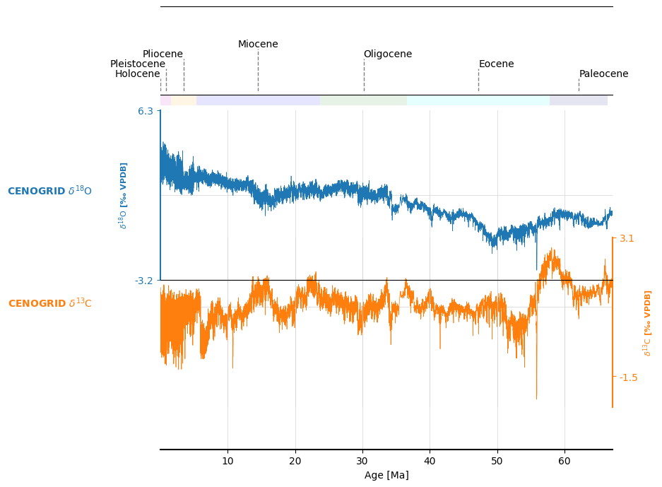
Adds the Geologic Time Scale (GTS) to the plot. :param fig: The figure object where the GTS will be added. :type fig: matplotlib.figure.Figure :param ax: The axis where the GTS will be plotted. :type ax: dict :param time_unit: Time units of the GTS data. Supported: ‘Ma’ (default), ‘ka’, ‘Ga’. :type time_unit: str :param GTS_df: DataFrame containing the GTS data with columns for ‘Rank’, ‘Name’, ‘Abbrev’, ‘Color’, ‘UpperBoundary’, ‘LowerBoundary’.
If None, the function will load the ICS chart from the provided URL.
- Parameters:
ranks (list of str, optional) – List of ranks to include (e.g., [‘Period’, ‘Epoch’, ‘Stage’]). If None, defaults to [‘Period’, ‘Epoch’, ‘Stage’]. Ranks are ordered from outer-most to inner-most.
location (str, optional) – Specifies whether to place the GTS above or below the plot. Default is ‘above’.
label_pref (str, optional) – Preference for labels: ‘full’ (default) for full names, ‘abbrev’ for abbreviations, ‘none’ for no labels (only colors).
allow_abbreviations (bool, optional) – If True, allows abbreviations for labels that don’t fit. Default is True.
lang (str, optional) – Language for GTS labels. Default is ‘en’.
ax_name (str, optional) – Name of the axis to create for the GTS. Default is ‘gts’.
v_offset (float, optional) – Vertical offset for the GTS labels. Default is 0.
height (float, optional) – Height of the GTS annotation area. Default is 0.05.
text_color (str or None, optional) – Color of the text labels. If None, the function will choose a contrasting color based on the bar color. Default is None.
fontsize (int, optional) – Font size for the GTS labels. Default is 12.
edgecolor (str, optional) – Color of the bar edges. Default is ‘k’ (black).
edgewidth (float, optional) – Width of the bar edges. Default is 0.
alpha (float, optional) – Transparency of the bars. Default is 1 (opaque).
zorder (int, optional) – Z-order for the GTS axis. Default is 10.
gts_url (str, optional) – URL to load the ICS chart if GTS_df is None. Default is the ICS chart URL.
- Returns:
fig (matplotlib.figure.Figure) – The figure object with the GTS added.
ax (dict) – The axis dictionary with the GTS axis added.
Examples
import pyleoclim as pyleo

ts_18 = pyleo.utils.load_dataset('cenogrid_d18O')
ts_13 = pyleo.utils.load_dataset('cenogrid_d13C')
ms = pyleo.MultipleSeries([ts_18, ts_13], label='Cenogrid', time_unit='ma BP')

fig, ax = ms.stackplot(figsize=(10, 5),linewidth=0.5, fill_between_alpha=0)
ax[0].invert_yaxis() # d18O is traditionally inverted

fig, ax = pyleo.utils.plotting.add_GTS(fig, ax, 'Ma', location='above', label_pref='full',
            allow_abbreviations=True, ax_name='gts', v_offset=0, height=.05)
Using rdflib to load GTS information from ICS
Time name: Age
Time unit: Ma

- pyleoclim.utils.plotting.calculate_overlapping_sets(fig, ax, labels, x_locs, fontsize, buffer=0.1)[source]
Calculate overlapping sets of labels based on their positions and widths.
This function identifies sets of labels that would overlap if rendered at the same height on a plot. It is used to determine how to place labels to avoid overlap in visualizations.
- Parameters:
ax (matplotlib.axes.Axes) – The Axes object on which the labels will be plotted.
labels (list of str) – A list of label strings.
x_locs (list of float) – A list of x-coordinates where the labels are to be positioned.
fontsize (int) – The font size used for the labels.
buffer (float, optional) – Additional space to consider around each label to prevent overlap. Defaults to 0.1.
- Returns:
list of list of int
- Return type:
A list where each sublist contains the indices of overlapping labels.
- pyleoclim.utils.plotting.closefig(fig=None)[source]
Close the figure
- Parameters:
fig (matplotlib.pyplot.figure) – The matplotlib figure object
- pyleoclim.utils.plotting.get_label_width(ax, label, buffer=0.0, fontsize=10)[source]
Helper function to find width of text when rendered in ax object
- pyleoclim.utils.plotting.highlight_intervals(ax, intervals, labels=None, color='g', alpha=0.3, legend=True)[source]
Hightlights intervals
This function highlights intervals.
- Parameters:
ax (matplotlib.axes.Axes object) –
intervals (list) – list of intervals to be highlighted
color (string or list) – If a string is passed, all intervals will be the specified color If a list is passed, the list is expected to be the same length as intervals
alpha (float or list) – If a float is passed, all intervals will have the same specified alpha value If a list is passed, the list is expected to be the same length as intervals
- Returns:
ax – the axis object from matplotlib See [matplotlib.axes](https://matplotlib.org/stable/api/axes_api.html) for details.
- Return type:
matplotlib.axis
Examples
import pyleoclim as pyleo

ts_18 = pyleo.utils.load_dataset('cenogrid_d18O')
ts_13 = pyleo.utils.load_dataset('cenogrid_d13C')
ms = pyleo.MultipleSeries([ts_18, ts_13], label='Cenogrid', time_unit='ma BP')

fig, ax = ms.stackplot(linewidth=0.5, fill_between_alpha=0)

ax=pyleo.utils.plotting.make_annotation_ax(fig, ax, ax_name = 'highlighted_intervals', zorder=-1)
intervals = [[3, 8], [12, 18], [30, 31], [40,43], [49, 60], [60, 65]]
ax['highlighted_intervals'] = pyleo.utils.plotting.highlight_intervals(ax['highlighted_intervals'], intervals,
    color='g', alpha=.1)

- pyleoclim.utils.plotting.infer_period_unit_from_time_unit(time_unit)[source]
infer a period unit based on the given time unit
- pyleoclim.utils.plotting.keep_center_colormap(cmap, vmin, vmax, center=0)[source]
Adjust a colormap so that a specific value remains centered, and extend its limits symmetrically.
This function modifies a given colormap such that the color representing the ‘center’ value remains at the center of the colormap. It does this by adjusting the minimum and maximum values symmetrically around the center and ensuring that the colormap covers a range that is at least 20% larger than the absolute range from the center to either the original minimum or maximum value. This is particularly useful for visualizing data with a significant central value (e.g., zero in anomaly maps) to ensure that the colormap visually represents deviations from this center in a balanced manner.
- Parameters:
cmap (str or Colormap) – The name of the colormap or a Colormap instance to be adjusted.
vmin (float) – The original minimum value in the data range that the colormap should cover.
vmax (float) – The original maximum value in the data range that the colormap should cover.
center (float, optional) – The value that should be centered in the adjusted colormap. Default is 0.
- Returns:
newmap – A new colormap instance adjusted so that ‘center’ is in the middle of the colormap, with its range symmetrically extended to ensure balanced representation of values around the center.
- Return type:
matplotlib.colors.ListedColormap
Notes
The adjustment involves shifting the original vmin and vmax values to be symmetric around the center, then expanding the range by at least 20% to ensure that the colormap’s central part accurately represents the centered value across the data. This adjusted colormap can then be used for data visualization tasks where maintaining a perceptual ‘zero’ or central reference point is important.
- pyleoclim.utils.plotting.label_intervals(fig, ax, labels, x_locs, orientation='north', overlapping_sets=None, baseline=0.5, height=0.5, buffer=0.1, fontsize=10, linewidth=None, linestyle_kwargs=None, text_kwargs=None)[source]
Place labels on a plot with given orientations and style parameters, avoiding overlaps.
This function positions labels at specified x-locations with adjustments to avoid overlaps. Labels can be oriented either above (north) or below (south) a baseline.
- Parameters:
ax (matplotlib.axes.Axes) – The Axes object where the labels are to be placed.
labels (list of str) – A list of label strings.
x_locs (list of float) – A list of x-coordinates for the labels.
orientation (str, optional) – The vertical orientation of the labels, either ‘north’ or ‘south’. Defaults to ‘north’.
overlapping_sets (list of list of int, optional) – Precomputed overlapping sets of labels. If None, the function will compute them. Defaults to None.
baseline (float, optional) – The baseline height for the first label slot. Defaults to 0.5.
height (float, optional) – The vertical spacing between slots. Defaults to 0.5.
buffer (float, optional) – Horizontal buffer space around labels to prevent overlap. Defaults to 0.1.
fontsize (int, optional) – Font size for labels. Defaults to 10.
linewidth (float, optional) – Line width for connecting lines. If None, defaults to 1.
linestyle_kwargs (dict, optional) – Additional keyword arguments for styling the connecting lines (per Matplotlib).
text_kwargs (dict, optional) – Additional keyword arguments for styling the text labels (per Matplotlib).
- Returns:
matplotlib.axes.Axes
- Return type:
The modified Axes object with labels placed.
Examples
import pyleoclim as pyleo
import numpy as np

ts_18 = pyleo.utils.load_dataset('cenogrid_d18O')
ts_13 = pyleo.utils.load_dataset('cenogrid_d13C')
ms = pyleo.MultipleSeries([ts_18, ts_13], label='Cenogrid', time_unit='ma BP')

fig, ax = ms.stackplot(linewidth=0.5, fill_between_alpha=0)

ax=pyleo.utils.plotting.make_annotation_ax(fig, ax, ax_name = 'epochs', height=.03,
                                   loc='above', v_offset=.015,zorder=-2)
ax['epochs'].set_facecolor((1, 1, 1, 0))

ceno_intervals_pairs = [[0.0, 0.01], [0.01, 1.6], [1.6, 5.3], [5.3, 23.7], [23.7, 36.6], [36.6, 57.8], [57.8, 66.4]]
ceno_epoch_labels = ['Holocene', 'Pleistocene', 'Pliocene', 'Miocene', 'Oligocene', 'Eocene', 'Paleocene']
ax['epochs'].set_ylim([-1,0])

colors = ['r', 'm', 'orange', 'blue', 'green', 'aqua', 'navy', 'pink']#['r', 'b']#'r' if ik%2 ==0 else 'b' for ik, _ts in enumerate(geo_ts)]
ax['epochs'] = pyleo.utils.plotting.highlight_intervals(ax['epochs'],
                                            ceno_intervals_pairs, color=colors,
                                                                      alpha=.1)

### EPOCHS (labels)
ax=pyleo.utils.plotting.make_annotation_ax(fig, ax['epochs'], ax_name = 'epoch_annotation',
                                           zorder=1, v_offset=0.01,
                                           height=.25, loc='above')

x_locs = [np.mean(interval) for interval in ceno_intervals_pairs]
ax['epoch_annotation'].set_ylim([0,3])
ax['epoch_annotation'] = pyleo.utils.plotting.label_intervals(fig, ax['epoch_annotation'], ceno_epoch_labels, x_locs,
                                                       orientation='north', baseline=.45, height=0.35, buffer=0.1,
                                   linestyle_kwargs= {'color':'gray'}, text_kwargs={'fontsize':10, 'va':'bottom'}
                                  )
- pyleoclim.utils.plotting.make_annotation_ax(fig, ax, loc='overlay', ax_name='highlighted_intervals', height=None, v_offset=0, b=None, width=None, h_offset=0, l=None, zorder=-1)[source]
Makes a clean axis for adding annotation
This function creates a new axes for adding annotation. If the bottom left corner is not specified, it is established based on the ax objects in ax. If there is only one ax object, this overkill, but is helpful to introduce annotations that span multiple data axes.
- Parameters:
ax (matplotlib.axes.Axes object or dict) – If ax is a dict, assumes data axes are assigned to integer keys and supplemental axes have string keys
loc (string) – if “overlay”, annotation ax will attempt to cover the area with data axes if “above”, annotation ax will be located directly above the top data ax if “below”, annotation ax will be located below the bottom data ax
ax_name (string) – name associated with new ax object
height (float) – height of annotation ax if loc = “above” or “below”, height=.025 if not specified if loc = “overlay”, height=vertical span of data axes, if not specified
v_offset (float) – vertical offset between data plot area and annotation ax a positive v_offset will place the bottom corner higher
width (float) – width of annotation ax horizontal span of data axes, if not specified
b (float) – location of bottom corner of annotation ax
h_offset (float) – horizontal offset from left corner a positive h_offset will place the left corner farther to the right
l (float) – location of left corner of annotation ax
zorder (numeric) – index of annotation ax layer in fig zorder = -1 will place the layer behind other layers zorder = 1000 will place the layer in front of other layers
- Returns:
ax_d – ax_d contains the original ax object(s) and new annotation ax assigned to specified ax_name See [matplotlib.axes](https://matplotlib.org/stable/api/axes_api.html) for details.
- Return type:
dict
- pyleoclim.utils.plotting.make_phantom_ax(ax)[source]
Remove all visual annotation from ax object
This function removes axis lines, axis labels, tick labels, tick marks and grid lines.
- Parameters:
ax (matplotlib.axes.Axes object) – the axes object to clear
- Returns:
ax – the axis object from matplotlib See [matplotlib.axes](https://matplotlib.org/stable/api/axes_api.html) for details.
- Return type:
matplotlib.axis
- pyleoclim.utils.plotting.make_scalar_mappable(cmap=None, hue_vect=None, n=None, norm_kwargs=None)[source]
Create a ScalarMappable object for mapping scalar data to colors.
This function configures and returns a ScalarMappable object based on the provided colormap (cmap), the scalar values (hue_vect), the number of discrete colors (n), and normalization parameters (norm_kwargs). It supports dynamic selection of normalization and colormap based on the input parameters and the range of scalar values.
- Parameters:
cmap (str, list, or None, optional) – The colormap to use for mapping scalar data to colors. Can be a name of a matplotlib colormap (str), a list of color names, or None. If None, defaults to ‘vlag’ if conditions for centered normalization are met, otherwise ‘viridis’.
hue_vect (np.ndarray, pd.Series, list, or None, optional) – An array-like object containing the scalar values to be mapped to colors. These values are used to determine the range and center for normalization.
n (int or None, optional) – Specifies the number of discrete colors in the colormap if cmap is provided as a list. If None, the number of colors is not explicitly set.
norm_kwargs (dict or None, optional) – A dictionary containing keyword arguments for the normalization process, specifically supporting ‘vcenter’ and ‘clip’. Defaults to {‘vcenter’: 0, ‘clip’: False} if not provided or if provided keys are missing.
- Returns:
ax_sm – The configured ScalarMappable object, which can be used to map scalar data to colors based on the specified colormap and normalization settings.
- Return type:
matplotlib.cm.ScalarMappable
Examples
import pyleoclim as pyleo
import numpy as np

scalar_values = np.random.randn(100)
sm = pyleo.utils.plotting.make_scalar_mappable(cmap='viridis', hue_vect=scalar_values)
# Now `sm` can be used with matplotlib plotting functions to map scalar values to colors.

sm = pyleo.utils.plotting.make_scalar_mappable(cmap='viridis', hue_vect=scalar_values, n=10)
# This creates a ScalarMappable a discrete color scale.

sm = pyleo.utils.plotting.make_scalar_mappable(cmap=['blue', 'white', 'red'], hue_vect=scalar_values, norm_kwargs={'vcenter': 0})
# This creates a ScalarMappable with a custom linear segmented colormap and centered normalization.
- pyleoclim.utils.plotting.plot_scatter_xy(x1, y1, x2, y2, figsize=None, xlabel=None, ylabel=None, title=None, xlim=None, ylim=None, savefig_settings=None, ax=None, legend=True, plot_kwargs=None, lgd_kwargs=None)[source]
Plot a scatter on top of a line plot.
- Parameters:
x1 (array) – x axis of timeseries1 - plotted as a line
y1 (array) – values of timeseries1 - plotted as a line
x2 (array) – x axis of scatter points
y2 (array) – y of scatter points
figsize (list) – a list of two integers indicating the figure size
xlabel (str) – label for x-axis
ylabel (str) – label for y-axis
title (str) – the title for the figure
xlim (list) – set the limits of the x axis
ylim (list) – set the limits of the y axis
ax (pyplot.axis) – the pyplot.axis object
legend (bool) – plot legend or not
lgd_kwargs (dict) – the keyword arguments for ax.legend()
plot_kwargs (dict) – the keyword arguments for ax.plot()
savefig_settings (dict) –
the dictionary of arguments for plt.savefig(); some notes below: - “path” must be specified; it can be any existing or non-existing path,
with or without a suffix; if the suffix is not given in “path”, it will follow “format”
”format” can be one of {“pdf”, “eps”, “png”, “ps”}
- Returns:
ax
- Return type:
the pyplot.axis object
See also
pyleoclim.utils.plotting.set_styleset different styles for the figures. Should be set before invoking the plotting functions
pyleoclim.utils.plotting.savefigsave figures
- pyleoclim.utils.plotting.plot_xy(x, y, figsize=None, xlabel=None, ylabel=None, title=None, xlim=None, ylim=None, savefig_settings=None, ax=None, legend=True, plot_kwargs=None, lgd_kwargs=None, invert_xaxis=False, invert_yaxis=False)[source]
Plot a timeseries
- Parameters:
x (array) – The time axis for the timeseries
y (array) – The values of the timeseries
figsize (list) – a list of two integers indicating the figure size
xlabel (str) – label for x-axis
ylabel (str) – label for y-axis
title (str) – the title for the figure
xlim (list) – set the limits of the x axis
ylim (list) – set the limits of the y axis
ax (pyplot.axis) – the pyplot.axis object
legend (bool) – plot legend or not
lgd_kwargs (dict) – the keyword arguments for ax.legend()
plot_kwargs (dict) – the keyword arguments for ax.plot()
mute (bool) –
if True, the plot will not show; recommend to turn on when more modifications are going to be made on ax
(going to be deprecated)
savefig_settings (dict) –
the dictionary of arguments for plt.savefig(); some notes below: - “path” must be specified; it can be any existing or non-existing path,
with or without a suffix; if the suffix is not given in “path”, it will follow “format”
”format” can be one of {“pdf”, “eps”, “png”, “ps”}
invert_xaxis (bool, optional) – if True, the x-axis of the plot will be inverted
invert_yaxis (bool, optional) – if True, the y-axis of the plot will be inverted
- Returns:
ax
- Return type:
the pyplot.axis object
See also
pyleoclim.utils.plotting.set_styleset different styles for the figures. Should be set before invoking the plotting functions
pyleoclim.utils.plotting.savefigsave figures
- pyleoclim.utils.plotting.savefig(fig, path=None, dpi=300, settings={}, verbose=True)[source]
Save a figure to a path
- Parameters:
fig (matplotlib.pyplot.figure) – the figure to save
path (str) – the path to save the figure, can be ignored and specify in “settings” instead
dpi (int) – resolution in dot (pixels) per inch. Default: 300.
settings (dict) –
the dictionary of arguments for plt.savefig(); some notes below: - “path” must be specified in settings if not assigned with the keyword argument;
it can be any existing or non-existing path, with or without a suffix; if the suffix is not given in “path”, it will follow “format”
”format” can be one of {“pdf”, “eps”, “png”, “ps”}
verbose (bool, {True,False}) – If True, print the path of the saved file.
- pyleoclim.utils.plotting.scatter_xy(x, y, c=None, figsize=None, xlabel=None, ylabel=None, title=None, xlim=None, ylim=None, savefig_settings=None, ax=None, legend=True, plot_kwargs=None, lgd_kwargs=None)[source]
Make scatter plot.
- Parameters:
x (numpy.array) – x value
y (numpy.array) – y value
c (array-like or list of colors or color, optional) – The marker colors. Possible values: - A scalar or sequence of n numbers to be mapped to colors using cmap and norm. - A 2D array in which the rows are RGB or RGBA. - A sequence of colors of length n. - A single color format string. Note that c should not be a single numeric RGB or RGBA sequence because that is indistinguishable from an array of values to be colormapped. If you want to specify the same RGB or RGBA value for all points, use a 2D array with a single row. Otherwise, value-matching will have precedence in case of a size matching with x and y. If you wish to specify a single color for all points prefer the color keyword argument. Defaults to None. In that case the marker color is determined by the value of color, facecolor or facecolors. In case those are not specified or None, the marker color is determined by the next color of the Axes’ current “shape and fill” color cycle. This cycle defaults to rcParams[“axes.prop_cycle”] (default: cycler(‘color’, [‘#1f77b4’, ‘#ff7f0e’, ‘#2ca02c’, ‘#d62728’, ‘#9467bd’, ‘#8c564b’, ‘#e377c2’, ‘#7f7f7f’, ‘#bcbd22’, ‘#17becf’])).
figsize (list, optional) – A list of two integers indicating the dimension of the figure. The default is None.
xlabel (str, optional) – x-axis label. The default is None.
ylabel (str, optional) – y-axis label. The default is None.
title (str, optional) – Title for the plot. The default is None.
xlim (list, optional) – Limits for the x-axis. The default is None.
ylim (list, optional) – Limits for the y-axis. The default is None.
savefig_settings (dict, optional) –
- the dictionary of arguments for plt.savefig(); some notes below:
”path” must be specified; it can be any existing or non-existing path, with or without a suffix; if the suffix is not given in “path”, it will follow “format”
”format” can be one of {“pdf”, “eps”, “png”, “ps”}
The default is None.
ax (pyplot.axis, optional) – The axis object. The default is None.
legend (bool, optional) – Whether to include a legend. The default is True.
plot_kwargs (dict, optional) – the keyword arguments for ax.plot(). The default is None.
lgd_kwargs (dict, optional) – the keyword arguments for ax.legend(). The default is None.
- Returns:
ax
- Return type:
the pyplot.axis object
- pyleoclim.utils.plotting.set_style(style='journal', font_scale=1.0, dpi=300)[source]
Modify the visualization style
This function is inspired by Seaborn.
- Parameters:
style ({journal,web,matplotlib,_spines, _nospines,_grid,_nogrid}) –
set the styles for the figure:
journal (default): fonts appropriate for paper
web: web-like font (e.g. ggplot)
matplotlib: the original matplotlib style
In addition, the following options are available:
_spines/_nospines: allow to show/hide spines
_grid/_nogrid: allow to show gridlines (default: _grid)
font_scale (float) – Default is 1. Corresponding to 12 Font Size.
- pyleoclim.utils.plotting.text_loc(fig, ax, rect, label_text, width, yloc)[source]
Determine if the label fits inside or outside the bar.
- Parameters:
fig (matplotlib.figure.Figure) – The figure object.
ax (matplotlib.axes.Axes) – The axis where the bar is plotted.
rect (matplotlib.patches.Rectangle) – The rectangle (bar) object.
label_text (str) – The text label to check.
width (float) – The width of the bar in data coordinates.
yloc (float) – The y location of the bar in data coordinates.
- Returns:
‘inside’ if the label fits inside the bar, ‘outside’ otherwise.
- Return type:
str
Spectral
Utilities for spectral analysis, including WWZ, CWT, Lomb-Scargle, MTM, and Welch. Designed for NumPy arrays, either evenly spaced or not (method-dependent).
All spectral methods must return a dictionary containing one vector for the frequency axis and the power spectral density (PSD).
Additional utilities help compute an optimal frequency vector or estimate scaling exponents.
- pyleoclim.utils.spectral.beta2Hurst(beta)[source]
Translates spectral slope to Hurst exponent
- Parameters:
beta (float) – the estimated slope of a power spectral density :math: S(f) propto 1/f^{beta}
- Returns:
H – Hurst index, should be in (0, 1)
- Return type:
float
See also
pyleoclim.utils.spectral.beta_estimationEstimate the scaling exponent of a power spectral density.
- pyleoclim.utils.spectral.beta_estimation(psd, freq, fmin=None, fmax=None, logf_binning_step='max', verbose=False)[source]
Estimate the scaling exponent of a power spectral density.
Models the spectrum as :math: S(f) propto 1/f^{beta}. For instance: - :math: beta = 0 corresponds to white noise - :math: beta = 1 corresponds to pink noise - :math: beta = 2 corresponds to red noise (Brownian motion)
- Parameters:
psd (array) – the power spectral density
freq (array) – the frequency vector
fmin (float) – the min of frequency range for beta estimation
fmax (float) – the max of frequency range for beta estimation
verbose (bool) – if True, will print out debug information
- Returns:
beta (float) – the estimated slope
f_binned (array) – binned frequency vector
psd_binned (array) – binned power spectral density
Y_reg (array) – prediction based on linear regression
- pyleoclim.utils.spectral.cwt_psd(ys, ts, freq=None, freq_method='log', freq_kwargs=None, scale=None, detrend=False, sg_kwargs={}, gaussianize=False, standardize=True, pad=False, mother='MORLET', param=None, cwt_res=None)[source]
Spectral estimation using the continuous wavelet transform Uses the Torrence and Compo [1998] continuous wavelet transform implementation
- Parameters:
ys (numpy.array) – the time series.
ts (numpy.array) – the time axis.
freq (numpy.array, optional) – The frequency vector. The default is None, which will prompt the use of one the underlying functions
freq_method (string, optional) – The method by which to obtain the frequency vector. The default is ‘log’. Options are ‘log’ (default), ‘nfft’, ‘lomb_scargle’, ‘welch’, and ‘scale’
freq_kwargs (dict, optional) – Optional parameters for the choice of the frequency vector. See make_freq_vector and additional methods for details. The default is {}.
scale (numpy.array) – Optional scale vector in place of a frequency vector. Default is None. If scale is not None, frequency method and attached arguments will be ignored.
detrend (bool, string, {'linear', 'constant', 'savitzy-golay', 'emd'}) – Whether to detrend and with which option. The default is False.
sg_kwargs (dict, optional) – Additional parameters for the savitzy-golay method. The default is {}.
gaussianize (bool, optional) – Whether to gaussianize. The default is False.
standardize (bool, optional) – Whether to standardize. The default is True.
pad (bool, optional) – Whether or not to pad the timeseries. with zeroes to get N up to the next higher power of 2. This prevents wraparound from the end of the time series to the beginning, and also speeds up the FFT’s used to do the wavelet transform. This will not eliminate all edge effects. The default is False.
mother (string, optional) – the mother wavelet function. The default is ‘MORLET’. Options are: ‘MORLET’, ‘PAUL’, or ‘DOG’
param (flaot, option) –
the mother wavelet parameter. The default is None since it varies for each mother
For ‘MORLET’ this is k0 (wavenumber), default is 6.
For ‘PAUL’ this is m (order), default is 4.
For ‘DOG’ this is m (m-th derivative), default is 2.
cwt_res (dict) – Results from pyleoclim.utils.wavelet.cwt
- Returns:
res –
- Dictionary containing:
psd: the power density function
freq: frequency vector
scale: the scale vector
mother: the mother wavelet
param : the wavelet parameter
- Return type:
dict
See also
pyleoclim.utils.wavelet.make_freq_vectormake the frequency vector with various methods
pyleoclim.utils.wavelet.cwtTorrence and Compo implementation of the continuous wavelet transform
pyleoclim.utils.spectral.periodogramSpectral estimation using Blackman-Tukey’s periodogram
pyleoclim.utils.spectral.mtmSpectral estimation using the multi-taper method
pyleoclim.utils.spectral.lomb_scargleSpectral estimation using the lomb-scargle periodogram
pyleoclim.utils.spectral.welchSpectral estimation using Welch’s periodogram
pyleoclim.utils.spectral.wwz_psdSpectral estimation using the Weighted Wavelet Z-transform
pyleoclim.utils.tsutils.detrenddetrending functionalities using 4 possible methods
pyleoclim.utils.tsutils.gaussianizeQuantile maps a 1D array to a Gaussian distribution
pyleoclim.utils.tsutils.standardizeCenters and normalizes a given time series.
References
Torrence, C. and G. P. Compo, 1998: A Practical Guide to Wavelet Analysis. Bull. Amer. Meteor. Soc., 79, 61-78. Python routines available at http://paos.colorado.edu/research/wavelets/
- pyleoclim.utils.spectral.lomb_scargle(ys, ts, freq=None, freq_method='lomb_scargle', freq_kwargs=None, n50=3, window='hann', detrend=None, sg_kwargs=None, gaussianize=False, standardize=True, average='mean')[source]
Lomb-scargle periodogram
Appropriate for unevenly-spaced arrays. Uses the lomb-scargle implementation: https://docs.scipy.org/doc/scipy/reference/generated/scipy.signal.lombscargle.html
- Parameters:
ys (array) – a time series
ts (array) – time axis of the time series
freq (str or array) – vector of frequency. If string, uses the following method:
freq_method (str) –
Method to generate the frequency vector if not set directly. The following options are avialable:
log
lomb_scargle (default)
welch
scale
nfft
See utils.wavelet.make_freq_vector for details
freq_kwargs (dict) – Arguments for the method chosen in freq_method. See specific functions in utils.wavelet for details By default, uses dt=median(ts), ofac=4 and hifac=1 for Lomb-Scargle
n50 (int) – The number of 50% overlapping segment to apply
window (str or tuple) –
Desired window to use. Possible values:
boxcar
triang
blackman
hamming
hann (default)
bartlett
flattop
parzen
bohman
blackmanharris
nuttail
barthann
kaiser (needs beta)
gaussian (needs standard deviation)
general_gaussian (needs power, width)
slepian (needs width)
dpss (needs normalized half-bandwidth)
chebwin (needs attenuation)
exponential (needs decay scale)
tukey (needs taper fraction)
If the window requires no parameters, then window can be a string. If the window requires parameters, then window must be a tuple with the first argument the string name of the window, and the next arguments the needed parameters. If window is a floating point number, it is interpreted as the beta parameter of the kaiser window.
detrend : str
If None, no detrending is applied. Available detrending methods:
None - no detrending will be applied (default);
linear - a linear least-squares fit to ys is subtracted;
constant - the mean of ys is subtracted
savitzy-golay - ys is filtered using the Savitzky-Golay filters and the resulting filtered series is subtracted from y.
emd - Empirical mode decomposition
sg_kwargs : dict
The parameters for the Savitzky-Golay filters. see pyleoclim.utils.filter.savitzy_golay for details.
gaussianize : bool
If True, gaussianizes the timeseries
standardize : bool
If True, standardizes the timeseriesprep_args : dict
average : {‘mean’,’median’}
Method to use when averaging periodograms. Defaults to ‘mean’.
- Returns:
res_dict – the result dictionary, including
freq (array): the frequency vector
psd (array): the spectral density vector
- Return type:
dict
See also
pyleoclim.utils.spectral.periodogramEstimate power spectral density using a periodogram
pyleoclim.utils.spectral.mtmRetuns spectral density using a multi-taper method
pyleoclim.utils.spectral.welchReturns power spectral density using the Welch method
pyleoclim.utils.spectral.wwz_psdSpectral estimation using the Weighted Wavelet Z-transform
pyleoclim.utils.spectral.cwt_psdSpectral estimation using the Continuous Wavelet Transform
pyleoclim.utils.filter.savitzy_golayFiltering using Savitzy-Golay
pyleoclim.utils.tsutils.detrenddetrending functionalities using 4 possible methods
pyleoclim.utils.tsutils.gaussianizeQuantile maps a 1D array to a Gaussian distribution
pyleoclim.utils.tsutils.standardizeCenters and normalizes a given time series.
References
Lomb, N. R. (1976). Least-squares frequency analysis of unequally spaced data. Astrophysics and Space Science 39, 447-462.
Scargle, J. D. (1982). Studies in astronomical time series analysis. II. Statistical aspects of spectral analyis of unvenly spaced data. The Astrophysical Journal, 263(2), 835-853.
- pyleoclim.utils.spectral.mtm(ys, ts, NW=None, BW=None, detrend=None, sg_kwargs=None, gaussianize=False, standardize=True, adaptive=False, jackknife=True, low_bias=True, sides='default', nfft=None)[source]
Spectral density using the multi-taper method.
If the NW product, or the BW and Fs in Hz are not specified by the user, a bandwidth of 4 times the fundamental frequency, corresponding to NW = 4 will be used.
Based on the nitime package: http://nipy.org/nitime/api/generated/nitime.algorithms.spectral.html
- Parameters:
ys (array) – a time series
ts (array) – time axis of the time series
NW (float) – The time-bandwidth product NW governs the width (and therefore, height) of a peak, which can take the values [2, 5/2, 3, 7/2, 4]. This product controls the classical bias-variance tradeoff inherent to spectral estimation: a large product limits the variance but increases leakage out of harmonic line. In other words, small values of NW mean high spectral resolution, low bias, but high variance. Large values of the parameter mean lower resolution, higher bias, but reduced variance. There is no automated way to choose this parameter, and the default (NW=4) corresponds to a conservative choice with low variance. For a demonstration on the effect of this parameter, see the spectral analysis notebook in our tutorials: https://pyleoclim-util.readthedocs.io/en/master/tutorials.html.
BW (float) – The sampling-relative bandwidth of the data tapers
detrend (str) –
- If None, no detrending is applied. Available detrending methods:
None - no detrending will be applied (default);
linear - a linear least-squares fit to ys is subtracted;
constant - the mean of ys is subtracted
savitzy-golay - ys is filtered using the Savitzky-Golay filters and the resulting filtered series is subtracted from y.
emd - Empirical mode decomposition
- sg_kwargsdict
The parameters for the Savitzky-Golay filters. see pyleoclim.utils.filter.savitzy_golay for details.
- gaussianizebool
If True, gaussianizes the timeseries
- standardizebool
If True, standardizes the timeseries
- adaptive{True/False}
Use an adaptive weighting routine to combine the PSD estimates of different tapers.
- jackknife{True/False}
Use the jackknife method to make an estimate of the PSD variance at each point.
- low_bias{True/False}
Rather than use 2NW tapers, only use the tapers that have better than 90% spectral concentration within the bandwidth (still using a maximum of 2NW tapers)
- sidesstr (optional) [ ‘default’ | ‘onesided’ | ‘twosided’ ]
This determines which sides of the spectrum to return. For complex-valued inputs, the default is two-sided, for real-valued inputs, default is one-sided Indicates whether to return a one-sided or two-sided
- Returns:
res_dict – the result dictionary, including - freq (array): the frequency vector - psd (array): the spectral density vector
- Return type:
dict
See also
pyleoclim.utils.spectral.periodogramSpectral density estimation using a Blackman-Tukey periodogram
pyleoclim.utils.spectral.welchspectral estimation using Welch’s periodogram
pyleoclim.utils.spectral.lomb_scargleLomb-scargle priodogram
pyleoclim.utils.spectral.wwz_psdSpectral estimation using the Weighted Wavelet Z-transform
pyleoclim.utils.spectral.cwt_psdSpectral estimation using the Continuous Wavelet Transform
pyleoclim.utils.filter.savitzy_golayFiltering using Savitzy-Golay
pyleoclim.utils.tsutils.detrenddetrending functionalities using 4 possible methods
pyleoclim.utils.tsutils.gaussianizeQuantile maps a 1D array to a Gaussian distribution
pyleoclim.utils.tsutils.standardizeCenters and normalizes a given time series.
- pyleoclim.utils.spectral.periodogram(ys, ts, window='hann', nfft=None, return_onesided=True, detrend=None, sg_kwargs=None, gaussianize=False, standardize=True, scaling='density')[source]
Spectral density estimation using a Blackman-Tukey periodogram
Based on the function from scipy.
- Parameters:
ys (array) – a time series
ts (array) – time axis of the time series
window (string or tuple) –
Desired window to use. Possible values:
boxcar (default)
triang
blackman
hamming
hann
bartlett
flattop
parzen
bohman
blackmanharris
nuttail
barthann
kaiser (needs beta)
gaussian (needs standard deviation)
general_gaussian (needs power, width)
slepian (needs width)
dpss (needs normalized half-bandwidth)
chebwin (needs attenuation)
exponential (needs decay scale)
tukey (needs taper fraction)
If the window requires no parameters, then window can be a string. If the window requires parameters, then window must be a tuple with the first argument the string name of the window, and the next arguments the needed parameters. If window is a floating point number, it is interpreted as the beta parameter of the kaiser window.
nfft (int) – Length of the FFT used, if a zero padded FFT is desired. If None, the FFT length is nperseg
return_onesided (bool) – If True, return a one-sided spectrum for real data. If False return a two-sided spectrum. Defaults to True, but for complex data, a two-sided spectrum is always returned.
detrend (str) –
If None, no detrending is applied. Available detrending methods:
None - no detrending will be applied (default);
linear - a linear least-squares fit to ys is subtracted;
constant - the mean of ys is subtracted
savitzy-golay - ys is filtered using the Savitzky-Golay filters and the resulting filtered series is subtracted from y.
emd - Empirical mode decomposition
sg_kwargs (dict) – The parameters for the Savitzky-Golay filters. see pyleoclim.utils.filter.savitzy_golay for details.
gaussianize (bool) – If True, gaussianizes the timeseries
standardize (bool) – If True, standardizes the timeseries
scaling ({"density,"spectrum}) – Selects between computing the power spectral density (‘density’) where Pxx has units of V**2/Hz and computing the power spectrum (‘spectrum’) where Pxx has units of V**2, if x is measured in V and fs is measured in Hz. Defaults to ‘density’
- Returns:
res_dict – the result dictionary, including
freq (array): the frequency vector
psd (array): the spectral density vector
- Return type:
dict
See also
pyleoclim.utils.spectral.welchEstimate power spectral density using the welch method
pyleoclim.utils.spectral.mtmRetuns spectral density using a multi-taper method
pyleoclim.utils.spectral.lomb_scargleReturn the computed periodogram using lomb-scargle algorithm
pyleoclim.utils.spectral.wwz_psdSpectral estimation using the Weighted Wavelet Z-transform
pyleoclim.utils.spectral.cwt_psdSpectral estimation using the Continuous Wavelet Transform
pyleoclim.utils.filter.savitzy_golayFiltering using Savitzy-Golay
pyleoclim.utils.tsutils.detrenddetrending functionalities using 4 possible methods
pyleoclim.utils.tsutils.gaussianizeQuantile maps a 1D array to a Gaussian distribution
pyleoclim.utils.tsutils.standardizeCenters and normalizes a given time series.
- pyleoclim.utils.spectral.psd_ar(var_noise, freq, ar_params, f_sampling)[source]
Theoretical power spectral density (PSD) of an autoregressive model
- Parameters:
var_noise (float) – the variance of the noise of the AR process
freq (array) – vector of frequency
ar_params (array) – autoregressive coefficients, not including zero-lag
f_sampling (float) – sampling frequency
- Returns:
psd – power spectral density
- Return type:
array
- pyleoclim.utils.spectral.psd_fBM(freq, ts, H)[source]
Theoretical power spectral density of a fractional Brownian motion
- Parameters:
freq (array) – vector of frequency
ts (array) – the time axis of the time series
H (float) – Hurst exponent, should be in (0, 1)
- Returns:
psd – power spectral density
- Return type:
array
References
Flandrin, P. On the spectrum of fractional Brownian motions. IEEE Transactions on Information Theory 35, 197–199 (1989).
- pyleoclim.utils.spectral.welch(ys, ts, window='hann', nperseg=None, noverlap=None, nfft=None, return_onesided=True, detrend=None, sg_kwargs=None, gaussianize=False, standardize=True, scaling='density', average='mean')[source]
Estimate power spectral density using Welch’s periodogram
Wrapper for the function implemented in scipy.signal.welch See https://docs.scipy.org/doc/scipy/reference/generated/scipy.signal.welch.html for details.
Welch’s method is an approach for spectral density estimation. It computes an estimate of the power spectral density by dividing the data into overlapping segments, computing a modified periodogram for each segment and averaging the periodograms to lower the estimator’s variance.
- Parameters:
ys (array) – a time series
ts (array) – time axis of the time series
window (string or tuple) –
Desired window to use. Possible values:
boxcar
triang
blackman
hamming
hann (default)
bartlett
flattop
parzen
bohman
blackmanharris
nuttail
barthann
kaiser (needs beta)
gaussian (needs standard deviation)
general_gaussian (needs power, width)
slepian (needs width)
dpss (needs normalized half-bandwidth)
chebwin (needs attenuation)
exponential (needs decay scale)
tukey (needs taper fraction)
If the window requires no parameters, then window can be a string. If the window requires parameters, then window must be a tuple with the first argument the string name of the window, and the next arguments the needed parameters. If window is a floating point number, it is interpreted as the beta parameter of the kaiser window.
nperseg (int) – Length of each segment. If none, nperseg=len(ys)/2. Default to None This will give three segments with 50% overlap
noverlap (int) – Number of points to overlap. If None, noverlap=nperseg//2. Defaults to None, represents 50% overlap
nfft (int) – Length of the FFT used, if a zero padded FFT is desired. If None, the FFT length is nperseg
return_onesided (bool) – If True, return a one-sided spectrum for real data. If False return a two-sided spectrum. Defaults to True, but for complex data, a two-sided spectrum is always returned.
detrend (str) –
If None, no detrending is applied. Available detrending methods:
None - no detrending will be applied (default);
linear - a linear least-squares fit to ys is subtracted;
constant - the mean of ys is subtracted
savitzy-golay - ys is filtered using the Savitzky-Golay filters and the resulting filtered series is subtracted from y.
emd - Empirical mode decomposition
sg_kwargs (dict) – The parameters for the Savitzky-Golay filters. see pyleoclim.utils.filter.savitzy_golay for details.
gaussianize (bool) – If True, gaussianizes the timeseries
standardize (bool) – If True, standardizes the timeseries
scaling ({"density,"spectrum}) – Selects between computing the power spectral density (‘density’) where Pxx has units of V**2/Hz and computing the power spectrum (‘spectrum’) where Pxx has units of V**2, if x is measured in V and fs is measured in Hz. Defaults to ‘density’
average ({'mean','median'}) – Method to use when combining periodograms. Defaults to ‘mean’.
- Returns:
res_dict – the result dictionary, including
freq (array): the frequency vector
psd (array): the spectral density vector
- Return type:
dict
See also
pyleoclim.utils.spectral.periodogramSpectral density estimation using a Blackman-Tukey periodogram
pyleoclim.utils.spectral.mtmSpectral density estimation using the multi-taper method
pyleoclim.utils.spectral.lomb_scargleLomb-scargle priodogram
pyleoclim.utils.spectral.wwz_psdSpectral estimation using the Weighted Wavelet Z-transform
pyleoclim.utils.spectral.cwt_psdSpectral estimation using the Continuous Wavelet Transform
pyleoclim.utils.filter.savitzy_golayFiltering using Savitzy-Golay
pyleoclim.utils.tsutils.detrenddetrending functionalities using 4 possible methods
pyleoclim.utils.tsutils.gaussianizeQuantile maps a 1D array to a Gaussian distribution
pyleoclim.utils.tsutils.standardizeCenters and normalizes a given time series.
References
- Welch, “The use of the fast Fourier transform for the estimation of power spectra:
A method based on time averaging over short, modified periodograms”, IEEE Trans. Audio Electroacoust. vol. 15, pp. 70-73, 1967.
- pyleoclim.utils.spectral.wwz_psd(ys, ts, freq=None, freq_method='log', freq_kwargs=None, tau=None, c=0.001, nproc=8, detrend=False, sg_kwargs=None, gaussianize=False, standardize=True, Neff_threshold=3, anti_alias=False, avgs=2, method='Kirchner_numba', wwa=None, wwz_Neffs=None, wwz_freq=None)[source]
Spectral estimation using the Weighted Wavelet Z-transform
The Weighted wavelet Z-transform (WWZ) is based on Morlet wavelet spectral estimation, using least squares minimization to suppress the energy leakage caused by data gaps. WWZ does not rely on interpolation or detrending, and is appropriate for unevenly-spaced datasets. In particular, we use the variant of Kirchner & Neal (2013), in which basis rotations mitigate the numerical instability that occurs in pathological cases with the original algorithm (Foster, 1996). The WWZ method has one adjustable parameter, a decay constant c that balances the time and frequency resolutions of the analysis. The smaller this constant is, the sharper the peaks. The default value is 1e-3 to obtain smooth spectra that lend themselves to better scaling exponent estimation, while still capturing the main periodicities.
Note that scalogram applications use the larger value (8π2)−1, justified elsewhere (Foster, 1996).
- Parameters:
ys (array) – a time series, NaNs will be deleted automatically
ts (array) – the time points, if ys contains any NaNs, some of the time points will be deleted accordingly
freq (array) – vector of frequency
freq_method (str, {'log', 'lomb_scargle', 'welch', 'scale', 'nfft'}) –
Method to generate the frequency vector if not set directly. The following options are avialable:
’log’ (default)
’lomb_scargle’
’welch’
’scale’
’nfft’
See
pyleoclim.utils.wavelet.make_freq_vector()for detailsfreq_kwargs (dict) – Arguments for the method chosen in freq_method. See specific functions in pyleoclim.utils.wavelet for details
tau (array) – the evenly-spaced time vector for the analysis, namely the time shift for wavelet analysis
c (float) – the decay constant that will determine the analytical resolution of frequency for analysis, the smaller the higher resolution; the default value 1e-3 is good for most of the spectral analysis cases
nproc (int) – the number of processes for multiprocessing
detrend (str, {None, 'linear', 'constant', 'savitzy-golay'}) –
Methods for detrending include:
None: the original time series is assumed to have no trend;
’linear’: a linear least-squares fit to ys is subtracted;
’constant’: the mean of ys is subtracted
’savitzy-golay’: ys is filtered using the Savitzky-Golay filters and the resulting filtered series is subtracted from y.
sg_kwargs (dict) – The parameters for the Savitzky-Golay filters. See
pyleoclim.utils.filter.savitzky_golay()for details.gaussianize (bool) – If True, gaussianizes the timeseries
standardize (bool) – If True, standardizes the timeseries
method (string, {'Foster', 'Kirchner', 'Kirchner_f2py', 'Kirchner_numba'}) –
Available specific implementation of WWZ include:
’Foster’: the original WWZ method;
’Kirchner’: the method Kirchner adapted from Foster;
’Kirchner_f2py’: the method Kirchner adapted from Foster, implemented with f2py for acceleration;
’Kirchner_numba’: the method Kirchner adapted from Foster, implemented with Numba for acceleration (default);
Neff_threshold (int) – threshold for the effective number of points
anti_alias (bool) – If True, uses anti-aliasing
avgs (int) – flag for whether spectrum is derived from instantaneous point measurements (avgs<>1) OR from measurements averaged over each sampling interval (avgs==1)
wwa (array) – the weighted wavelet amplitude, returned from pyleoclim.utils.wavelet.wwz
wwz_Neffs (array) – the matrix of effective number of points in the time-scale coordinates, returned from pyleoclim.utils.wavelet.wwz
wwz_freq (array) – the returned frequency vector from pyleoclim.utils.wavelet.wwz
- Returns:
res (namedtuple) – a namedtuple that includes below items
psd (array) – power spectral density
freq (array) – vector of frequency
See also
pyleoclim.utils.spectral.periodogramEstimate power spectral density using a periodogram
pyleoclim.utils.spectral.mtmRetuns spectral density using a multi-taper method
pyleoclim.utils.spectral.lomb_scargleReturn the computed periodogram using lomb-scargle algorithm
pyleoclim.utils.spectral.welchEstimate power spectral density using the Welch method
pyleoclim.utils.spectral.cwt_psdSpectral estimation using the Continuous Wavelet Transform
pyleoclim.utils.filter.savitzy_golayFiltering using Savitzy-Golay
pyleoclim.utils.tsutils.detrenddetrending functionalities using 4 possible methods
pyleoclim.utils.tsutils.gaussianizeQuantile maps a 1D array to a Gaussian distribution
pyleoclim.utils.tsutils.standardizeCenters and normalizes a given time series.
References
Foster, G. (1996). Wavelets for period analysis of unevenly sampled time series. The Astronomical Journal, 112(4), 1709-1729.
Kirchner, J. W. (2005). Aliasin in 1/f^a noise spectra: origins, consequences, and remedies. Physical Review E covering statistical, nonlinear, biological, and soft matter physics, 71, 66110.
Kirchner, J. W. and Neal, C. (2013). Universal fractal scaling in stream chemistry and its impli-cations for solute transport and water quality trend detection. Proc Natl Acad Sci USA 110:12213–12218.
Tsmodel
Module for timeseries modeling
- pyleoclim.utils.tsmodel.ar1_fit(y, t=None)[source]
Return lag-1 autocorrelation
Returns the lag-1 autocorrelation from AR(1) fit OR persistence from tauest.
- Parameters:
y (array) – The time series
t (array) – The time axis of that series
- Returns:
g – Lag-1 autocorrelation coefficient (for evenly-spaced time series) OR estimated persistence (for unevenly-spaced time series)
- Return type:
float
See also
pyleoclim.utils.tsbase.is_evenly_spacedCheck if a time axis is evenly spaced, within a given tolerance
pyleoclim.utils.tsmodel.tau_estimationEstimates the temporal decay scale of an (un)evenly spaced time series.
- pyleoclim.utils.tsmodel.ar1_fit_evenly(y)[source]
Returns the lag-1 autocorrelation from AR(1) fit.
Uses statsmodels.tsa.arima.model.ARIMA. to calculate lag-1 autocorrelation
MARK FOR DEPRECATION once uar1_fit is adopted
- Parameters:
y (array) – Vector of (float) numbers as a time series
- Returns:
g – Lag-1 autocorrelation coefficient
- Return type:
float
- pyleoclim.utils.tsmodel.ar1_model(t, tau, output_sigma=1)[source]
Simulate AR(1) process with REDFIT
Simulate a (possibly irregularly-sampled) AR(1) process with given decay constant tau, à la REDFIT.
- Parameters:
t (array) – Time axis of the time series
tau (float) – The averaged persistence
- Returns:
y – The AR(1) time series
- Return type:
array
References
- Schulz, M. & Mudelsee, M. REDFIT: estimating red-noise spectra directly from unevenly spaced
paleoclimatic time series. Computers & Geosciences 28, 421–426 (2002).
- pyleoclim.utils.tsmodel.ar1_sim(y, p, t=None)[source]
Simulate AR(1) process(es) with sample autocorrelation value
Produce p realizations of an AR(1) process of length n with lag-1 autocorrelation g calculated from y and (if provided) t
Will be replaced by uar1_sim in a future release
- Parameters:
y (array) – a time series; NaNs not allowed
p (int) – column dimension (number of surrogates)
t (array) – the time axis of the series
- Returns:
ysim – n by p matrix of simulated AR(1) vector
- Return type:
array
See also
pyleoclim.utils.tsmodel.ar1_modelSimulates a (possibly irregularly-sampled) AR(1) process with given decay constant tau, à la REDFIT.
pyleoclim.utils.tsmodel.ar1_fitReturns the lag-1 autocorrelation from AR(1) fit OR persistence from tauest.
pyleoclim.utils.tsmodel.ar1_fit_evenlyReturns the lag-1 autocorrelation from AR(1) fit assuming even temporal spacing.
pyleoclim.utils.tsmodel.tau_estimationEstimates the temporal decay scale of an (un)evenly spaced time series.
- pyleoclim.utils.tsmodel.colored_noise(alpha, t, std=1.0, f0=None, m=None, seed=None)[source]
Generate a colored noise timeseries
- Parameters:
alpha (float) – exponent of the 1/f^alpha noise
t (float) – time vector of the generated noise
std (float) – standard deviation of the series. defaults to 1.0
f0 (float) – fundamental frequency
m (int) – maximum number of the waves, which determines the highest frequency of the components in the synthetic noise
seed (int) – seed for the random number generator
- Returns:
y – the generated 1/f^alpha noise
- Return type:
array
See also
pyleoclim.utils.tsmodel.gen_tsGenerate pyleoclim.Series with timeseries models
References
Eq. (15) in Kirchner, J. W. Aliasing in 1/f(alpha) noise spectra: origins, consequences, and remedies. Phys Rev E Stat Nonlin Soft Matter Phys 71, 066110 (2005).
- pyleoclim.utils.tsmodel.colored_noise_2regimes(alpha1, alpha2, f_break, t, f0=None, m=None, seed=None)[source]
Generate a colored noise timeseries with two regimes
- Parameters:
alpha1 (float) – the exponent of the 1/f^alpha noise
alpha2 (float) – the exponent of the 1/f^alpha noise
f_break (float) – the frequency where the scaling breaks
t (float) – time vector of the generated noise
f0 (float) – fundamental frequency
m (int) – maximum number of the waves, which determines the highest frequency of the components in the synthetic noise
- Returns:
y – the generated 1/f^alpha noise
- Return type:
array
See also
pyleoclim.utils.tsmodel.gen_tsGenerate pyleoclim.Series with timeseries models
References
Eq. (15) in Kirchner, J. W. Aliasing in 1/f(alpha) noise spectra: origins, consequences, and remedies. Phys Rev E Stat Nonlin Soft Matter Phys 71, 066110 (2005).
- pyleoclim.utils.tsmodel.gen_ar1_evenly(t, g, scale=1, burnin=50)[source]
Generate AR(1) series samples
MARK FOR DEPRECATION once uar1_fit is adopted
Wrapper for the function statsmodels.tsa.arima_process.arma_generate_sample. used to generate an ARMA
- Parameters:
t (array) – the time axis
g (float) – lag-1 autocorrelation
scale (float) – The standard deviation of the noise.
burnin (int) – Number of observation at the beginning of the sample to drop. Used to reduce dependence on initial values.
- Returns:
y – the generated AR(1) series
- Return type:
array
See also
pyleoclim.utils.tsmodel.gen_tsGenerate pyleoclim.Series with timeseries models
- pyleoclim.utils.tsmodel.gen_ts(model, t=None, nt=1000, **kwargs)[source]
Generate pyleoclim.Series with timeseries models
- Parameters:
model (str, {'colored_noise', 'colored_noise_2regimes', 'ar1'}) –
the timeseries model to use
colored_noise : colored noise with one scaling slope
colored_noise_2regimes : colored noise with two regimes of two different scaling slopes
ar1 : AR(1) series, with default autocorrelation of 0.5
t (array) – the time axis
nt (number of time points) – only works if ‘t’ is None, and it will use an evenly-spaced vector with nt points
kwargs (dict) – the keyward arguments for the specified timeseries model
- Returns:
t, v – time axis and values
- Return type:
NumPy arrays
See also
pyleoclim.utils.tsmodel.colored_noiseGenerate a colored noise timeseries
pyleoclim.utils.tsmodel.colored_noise_2regimesGenerate a colored noise timeseries with two regimes
pyleoclim.utils.tsmodel.gen_ar1_evenlyGenerate an AR(1) series
- pyleoclim.utils.tsmodel.isopersistent_rn(y, p)[source]
Generates p realization of a red noise [i.e. AR(1)] process with same persistence properties as y (Mean and variance are also preserved).
- Parameters:
X (array) – vector of (real) numbers as a time series, no NaNs allowed
p (int) – number of simulations
- Returns:
red (numpy array) – n rows by p columns matrix of an AR1 process, where n is the size of X
g (float) – lag-1 autocorrelation coefficient
See also
pyleoclim.utils.correlation.fdrDetermine significance based on the false discovery rate
Notes
(Some Rights Reserved) Hepta Technologies, 2008
- pyleoclim.utils.tsmodel.n_ll_unevenly_spaced_ar1(theta, y, t)[source]
Compute the negative log-likelihood of an evenly/unevenly spaced AR(1) model. It is assumed that the vector theta is initialized with log of tau and log of sigma 2.
- Parameters:
theta (array, length 2) – the first value is tau, the second value sigma^2.
y (array,length n) – The vector of observations.
t (array,length n,) – the vector of time values.
- Return type:
float. The value of the negative log likelihood evalued with the arguments provided (theta, y, t).
- pyleoclim.utils.tsmodel.random_time_axis(n, delta_t_dist='exponential', param=[1.0], seed=None)[source]
Generate a random time axis according to a specific probability model
- Parameters:
n (integer) – The length of the time series
delta_t_dist (str) –
the probability distribution of the random time increments. possible choices include ‘exponential’, ‘poisson’, ‘pareto’, or ‘random_choice’.
if ‘exponential’, param is expected to be a single scale parameter (traditionally denoted lambda) if ‘poisson’, param is expected to be a single parameter (rate) if ‘pareto’, expects a 2-list with 2 scalar shape & scale parameters (in that order) if ‘random_choice’, expects a 2-list containing the arrays:
- value_random_choice:
elements from which the random sample is generated (e.g. [1,2])
- prob_random_choice:
probabilities associated with each entry value_random_choice (e.g. [.95,.05])
(These two arrays must be of the same size)
- Returns:
t
- Return type:
1D array of random time axis obtained by taking the cumulative sum of the sampled random time increments, length n
- pyleoclim.utils.tsmodel.sm_ar1_sim(n, p, g, sig)[source]
Produce p realizations of an AR1 process of length n with lag-1 autocorrelation g using statsmodels
- Parameters:
n (int) – row dimensions
p (int) – column dimensions
g (float) – lag-1 autocorrelation coefficient
sig (float) – the standard deviation of the original time series
- Returns:
red – n rows by p columns matrix of an AR1 process
- Return type:
numpy matrix
See also
pyleoclim.utils.correlation.fdrDetermine significance based on the false discovery rate
- pyleoclim.utils.tsmodel.tau_estimation(y, t)[source]
Estimates the temporal decay scale of an (un)evenly spaced time series.
Esimtates the temporal decay scale of an (un)evenly spaced time series. Uses scipy.optimize.minimize_scalar.
- Parameters:
y (array) – A time series
t (array) – Time axis of the time series
- Returns:
tau_est – The estimated persistence
- Return type:
float
References
- Mudelsee, M. TAUEST: A Computer Program for Estimating Persistence in Unevenly Spaced Weather/Climate Time Series.
Comput. Geosci. 28, 69–72 (2002).
- pyleoclim.utils.tsmodel.uar1_fit(y, t)[source]
Maximum Likelihood Estimation of parameters tau and sigma_2
- Parameters:
y (An array of the values of the time series) – Values of the times series.
t (An array of the time index values of the time series) – Time index values of the time series
- Returns:
theta_hat
- Return type:
An array containing the estimated parameters tau_hat and sigma_2_hat, first entry is tau_hat, second entry is sigma_2_hat
- pyleoclim.utils.tsmodel.uar1_sim(t, tau, sigma_2=1)[source]
Generate a time series of length n from an autoregressive process of order 1 with evenly/unevenly spaced time points.
- Parameters:
t (array) – Time axis
tau (float) – Time decay parameter of the AR(1) model ($phi = e^{-tau}$)
sigma_2 (float) – Variance of the innovations
- Returns:
ys – matrix of simulated AR(1) vector
- Return type:
n
See also
pyleoclim.utils.tsmodel.uar1_fitMaximumum likelihood estimate of AR(1) parameters
Wavelet
Utilities for wavelet analysis, including Weighted Wavelet Z-transform (WWZ) and Continuous Wavelet Transform (CWT) à la Torrence & Compo 1998.
Includes multiple options for WWZ (Fortran via f2py, numba, multiprocessing) and enables cross-wavelet transform with either WWZ or CWT.
Designed for NumPy arrays, either evenly spaced or not (method-dependent)
- class pyleoclim.utils.wavelet.AliasFilter[source]
Performing anti-alias filter on a psd
experimental: Use at your own risk
@author: fzhu
- alias_filter(freq, pwr, fs, fc, f_limit, avgs)[source]
The anti-aliasing filter
- Parameters:
freq (array) – vector of frequencies in power spectrum
pwr (array) – vector of spectral power corresponding to frequencies “freq”
fs (float) – sampling frequency
fc (float) – corner frequency for 1/f^2 steepening of power spectrum
f_limit (float) – lower frequency limit for estimating misfit of model-plus-alias spectrum vs. measured power
avgs (int) – flag for whether spectrum is derived from instantaneous point measurements (avgs<>1) OR from measurements averaged over each sampling interval (avgs==1)
- Returns:
alpha (float) – best-fit exponent of power-law model
filtered_pwr (array) – vector of alias-filtered spectral power
model_pwr (array) – vector of modeled spectral power
aliased_pwr (array) – vector of modeled spectral power, plus aliases
References
Kirchner, J. W. Aliasing in 1/f(alpha) noise spectra: origins, consequences, and remedies. Phys Rev E Stat Nonlin Soft Matter Phys 71, 66110 (2005).
- pyleoclim.utils.wavelet.angle_sig(theta, nMC=1000, level=0.05)[source]
Calculates the mean angle and assesses the significance of its statistics.
In general, a consistent phase relationship will have low circular standard deviation (sigma <= sigma_lo) and high concentration (kappa >= kappa_hi).
- Parameters:
theta (numpy.array) – array of phase angles
nMC (int) – number of Monte Carlo simulations to assess angle confidence interval if None, the simulation is not performed.
level (float) – significance level against which to gauge sigma and kappa. default: 0.05
- Returns:
angle_mean (float) – mean angle
sigma (float) – circular standard deviation
kappa (float) – an estimate of the Von Mises distribution’s kappa parameter. kappa is a measure of concentration (a reciprocal measure of dispersion, so 1/kappa is analogous to the variance).
sigma_lo (float) – alpha-level quantile for sigma
kappa_hi (float) – (1-alpha)-level quantile for kappa
References
_[1] Grinsted, A., J. C. Moore, and S. Jevrejeva (2004), Application of the cross wavelet transform and wavelet coherence to geophysical time series, Nonlinear Processes in Geophysics, 11, 561–566.
_[2] Huber, R., Dutra, L. V., & da Costa Freitas, C. (2001, July). SAR interferogram phase filtering based on the Von Mises distribution. In IGARSS 2001. Scanning the Present and Resolving the Future. Proceedings. IEEE 2001 International Geoscience and Remote Sensing Symposium (Cat. No. 01CH37217) (Vol. 6, pp. 2816-2818). IEEE.
See also
pyleoclim.utils.wavelet.angle_statsphase angle statistics
- pyleoclim.utils.wavelet.angle_stats(theta)[source]
Statistics of a phase angle
- Parameters:
theta (numpy.array) – array of phase angles
- Returns:
mean_theta (float) – mean angle
sigma (float) – circular standard deviation
kappa (float) – an estimate of the Von Mises distribution’s kappa parameter
References
_[1] Huber, R., Dutra, L. V., & da Costa Freitas, C. (2001, July). SAR interferogram phase filtering based on the Von Mises distribution. In IGARSS 2001. Scanning the Present and Resolving the Future. Proceedings. IEEE 2001 International Geoscience and Remote Sensing Symposium (Cat. No. 01CH37217) (Vol. 6, pp. 2816-2818). IEEE.
See also
pyleoclim.utils.wavelet.angle_sigsignificance of phase angle statistics
- pyleoclim.utils.wavelet.assertPositiveInt(*args)[source]
Assert that the arguments are all integers larger than unity
- Parameters:
args –
- pyleoclim.utils.wavelet.chisquare_inv(P, V)[source]
Returns the inverse of chi-square CDF with V degrees of freedom at fraction P
- Parameters:
P (float) – fraction
V (float) – degress of freedom
- Returns:
X – Inverse chi-square
- Return type:
float
References
Torrence, C. and G. P. Compo, 1998: A Practical Guide to Wavelet Analysis. Bull. Amer. Meteor. Soc., 79, 61-78. Python routines available at http://paos.colorado.edu/research/wavelets/
- pyleoclim.utils.wavelet.chisquare_solve(XGUESS, P, V)[source]
Given XGUESS, a percentile P, and degrees-of-freedom V, return the difference between calculated percentile and P.
- Parameters:
XGUESS (float) – sig level
P (float) – percentile
V (float) – degrees of freedom
- Returns:
PDIFF – difference between calculated percentile and P
- Return type:
float
References
Torrence, C. and G. P. Compo, 1998: A Practical Guide to Wavelet Analysis. Bull. Amer. Meteor. Soc., 79, 61-78. Python routines available at http://paos.colorado.edu/research/wavelets/
- pyleoclim.utils.wavelet.cwt(ys, ts, freq=None, freq_method='log', freq_kwargs={}, scale=None, detrend=False, sg_kwargs={}, gaussianize=False, standardize=True, pad=False, mother='MORLET', param=None)[source]
Wrapper function to implement Torrence and Compo continuous wavelet transform
- Parameters:
ys (numpy.array) – the time series.
ts (numpy.array) – the time axis.
freq (numpy.array, optional) – The frequency vector. The default is None, which will prompt the use of one the underlying functions
freq_method (string, optional) – The method by which to obtain the frequency vector. The default is ‘log’. Options are ‘log’ (default), ‘nfft’, ‘lomb_scargle’, ‘welch’, and ‘scale’
freq_kwargs (dict, optional) – Optional parameters for the choice of the frequency vector. See make_freq_vector and additional methods for details. The default is {}.
scale (numpy.array) – Optional scale vector in place of a frequency vector. Default is None. If scale is not None, frequency method and attached arguments will be ignored.
detrend (bool, string, {'linear', 'constant', 'savitzy-golay', 'emd'}) – Whether to detrend and with which option. The default is False.
sg_kwargs (dict, optional) – Additional parameters for the savitzy-golay method. The default is {}.
gaussianize (bool, optional) – Whether to gaussianize. The default is False.
standardize (bool, optional) – Whether to standardize. The default is True.
pad (bool, optional) – Whether or not to pad the timeseries. with zeroes to get N up to the next higher power of 2. This prevents wraparound from the end of the time series to the beginning, and also speeds up the FFT’s used to do the wavelet transform. This will not eliminate all edge effects. The default is False.
mother (string, optional) – the mother wavelet function. The default is ‘MORLET’. Options are: ‘MORLET’, ‘PAUL’, or ‘DOG’
param (flaot, optional) –
- the mother wavelet parameter. The default is None since it varies for each mother
For ‘MORLET’ this is k0 (wavenumber), default is 6.
For ‘PAUL’ this is m (order), default is 4.
For ‘DOG’ this is m (m-th derivative), default is 2.
- Returns:
res –
- Dictionary containing:
amplitude: the wavelet amplitude
coi: cone of influence
freq: frequency vector
coeff: the wavelet coefficients
scale: the scale vector
time: the time vector
mother: the mother wavelet
param : the wavelet parameter
- Return type:
dict
See also
pyleoclim.utils.wavelet.make_freq_vectormake the frequency vector with various methods
pyleoclim.utils.wavelet.tc_waveletthe underlying wavelet function by Torrence and Compo
pyleoclim.utils.tsutils.detrenddetrending functionalities
pyleoclim.utils.tsutils.gaussianizeQuantile maps a 1D array to a Gaussian distribution
pyleoclim.utils.tsutils.preprocesspre-processes a times series using Gaussianization and detrending.
References
Torrence, C. and G. P. Compo, 1998: A Practical Guide to Wavelet Analysis. Bull. Amer. Meteor. Soc., 79, 61-78. Python routines available at http://paos.colorado.edu/research/wavelets/
- pyleoclim.utils.wavelet.cwt_coherence(y1, t1, y2, t2, freq=None, freq_method='log', freq_kwargs={}, scale=None, detrend=False, sg_kwargs={}, pad=False, standardize=True, gaussianize=False, tau=None, Neff_threshold=3, mother='MORLET', param=None, smooth_factor=0.25)[source]
Returns the wavelet transform coherency of two time series using the CWT.
- Parameters:
y1 (array) – first of two time series
y2 (array) – second of the two time series
t1 (array) – time axis of first time series
t2 (array) – time axis of the second time series (should be = t1)
tau (array) – evenly-spaced time points at which to evaluate coherence Defaults to None, which uses t1
freq (array) – vector of frequency
freq_method (string, optional) – The method by which to obtain the frequency vector. The default is ‘log’. Options are ‘log’ (default), ‘nfft’, ‘lomb_scargle’, ‘welch’, and ‘scale’
freq_kwargs (dict, optional) – Optional parameters for the choice of the frequency vector. See make_freq_vector and additional methods for details. The default is {}.
scale (numpy.array) – Optional scale vector in place of a frequency vector. Default is None. If scale is not None, frequency method and attached arguments will be ignored.
detrend (bool, string, {'linear', 'constant', 'savitzy-golay', 'emd'}) – Whether to detrend and with which option. The default is False.
sg_kwargs (dict, optional) – Additional parameters for the savitzy-golay method. The default is {}.
gaussianize (bool, optional) – Whether to gaussianize. The default is False.
standardize (bool, optional) – Whether to standardize. The default is True.
pad (bool, optional) – Whether or not to pad the timeseries with zeroes to increase N to the next higher power of 2. This prevents wraparound from the end of the time series to the beginning, and also speeds up the FFT used to do the wavelet transform. This will not eliminate all edge effects. The default is False.
mother (string, optional) – the mother wavelet function. The default is ‘MORLET’. Options are: ‘MORLET’, ‘PAUL’, or ‘DOG’
param (float, optional) –
- the mother wavelet parameter. The default is None since it varies for each mother
For ‘MORLET’ this is k0 (wavenumber), default is 6.
For ‘PAUL’ this is m (order), default is 4.
For ‘DOG’ this is m (m-th derivative), default is 2.
smooth_factor (float) – smoothing factor for the WTC (default: 0.25)
Neff_threshold (int) – threshold for the effective number of points (3 by default, see make_coi())
- Returns:
res – contains the cross wavelet coherence (WTC), cross-wavelet transform (XWT), cross-wavelet phase, vector of frequency, evenly-spaced time points, nMC AR1 scalograms, cone of influence.
- Return type:
dict
References
Grinsted, A., J. C. Moore, and S. Jevrejeva (2004), Application of the cross wavelet transform and wavelet coherence to geophysical time series, Nonlinear Processes in Geophysics, 11, 561–566.
See also
pyleoclim.utils.wavelet.cwtContinuous Wavelet Transform (Torrence & Compo 1998)
pyleoclim.utils.filter.savitzky_golaySmooth (and optionally differentiate) data with a Savitzky-Golay filter.
pyleoclim.utils.wavelet.make_freq_vectorMakes frequency vector
pyleoclim.utils.tsutils.gaussianizeQuantile maps a 1D array to a Gaussian distribution
pyleoclim.utils.tsutils.detrenddetrending functionalities
pyleoclim.utils.tsutils.preprocesspre-processes a times series using Gaussianization and detrending.
- pyleoclim.utils.wavelet.freq_vector_log(ts, fmin=None, fmax=None, nf=None)[source]
Return the frequency vector based on logspace
- Parameters:
ts (array) – time axis of the time series
fmin (float) – minimum frequency. If None is provided (default), inferred by the method.
fmax (float) – maximum frequency. If None is provided (default), inferred by the method.
nf (int) – number of freq points. If None is provided, defaults to ceil(N/10).
- Returns:
freq – the frequency vector
- Return type:
array
See also
pyleoclim.utils.wavelet.freq_vector_lomb_scargleReturn the frequency vector based on the REDFIT recommendation.
pyleoclim.utils.wavelet.freq_vector_welchReturn the frequency vector based on the Welch’s method.
pyleoclim.utils.wavelet.freq_vector_nfftReturn the frequency vector based on NFFT
pyleoclim.utils.wavelet.freq_vector_scaleReturn the frequency vector based on scales
pyleoclim.utils.wavelet.make_freq_vectorMake frequency vector
- pyleoclim.utils.wavelet.freq_vector_lomb_scargle(ts, dt=None, nf=None, ofac=4, hifac=0.95)[source]
Return the frequency vector based on the REDFIT recommendation.
- Parameters:
ts (array) – time axis of the time series
dt (float) – The resolution of the data. If None, uses the median resolution. Defaults to None.
nf (int) – Number of frequency points. If None, calculated as the difference between the highest and lowest frequencies (set by hifac and ofac) divided by resolution. Defaults to None
ofac (float) –
- Oversampling rate that influences the resolution of the frequency axis,
when equals to 1, it means no oversamling (should be >= 1). The default value 4 is usually a good value.
hifac (float) – fhi/fnyq (should be <= 1), where fhi is the highest frequency that can be analyzed by the Lomb-Scargle algorithm and fnyq is the Nyquist frequency.
- Returns:
freq – the frequency vector
- Return type:
array
References
Trauth, M. H. MATLAB® Recipes for Earth Sciences. (Springer, 2015). pp 181.
See also
pyleoclim.utils.wavelet.freq_vector_welchReturn the frequency vector based on the Welch’s method.
pyleoclim.utils.wavelet.freq_vector_nfftReturn the frequency vector based on NFFT
pyleoclim.utils.wavelet.freq_vector_scaleReturn the frequency vector based on scales
pyleoclim.utils.wavelet.freq_vector_logReturn the frequency vector based on logspace
pyleoclim.utils.wavelet.make_freq_vectorMake frequency vector
- pyleoclim.utils.wavelet.freq_vector_nfft(ts)[source]
Return the frequency vector based on NFFT
- Parameters:
ts (array) – time axis of the time series
- Returns:
freq – the frequency vector
- Return type:
array
See also
pyleoclim.utils.wavelet.freq_vector_lomb_scargleReturn the frequency vector based on the REDFIT recommendation.
pyleoclim.utils.wavelet.freq_vector_welchReturn the frequency vector based on the Welch’s method.
pyleoclim.utils.wavelet.freq_vector_scaleReturn the frequency vector based on scales
pyleoclim.utils.wavelet.freq_vector_logReturn the frequency vector based on logspace
pyleoclim.utils.wavelet.make_freq_vectorMake frequency vector
- pyleoclim.utils.wavelet.freq_vector_scale(ts, dj=0.25, s0=None, j1=None, mother='MORLET', param=None)[source]
Return the frequency vector based on scales for wavelet analysis. This function is adapted from Torrence and Compo [1998]
- Parameters:
ts (numpy.array) – The time axis for the timeseries
dj (float, optional) – The spacing between discrete scales. The default is 0.25. A smaller number will give better scale resolution, but be slower to plot.
s0 (float, optional) – the smallest scale of the wavelet. The default is None, representing 2*dT.
j1 (float, optional) – the number of scales minus one. Scales range from S0 up to S0*2**(J1*DJ), to give a total of (J1+1) scales. The default is None, which represents (LOG2(N DT/S0))/DJ.
mother (string, optional) – the mother wavelet function. The default is ‘MORLET’. Options are: ‘MORLET’, ‘PAUL’, or ‘DOG’
param (flaot, optional) –
the mother wavelet parameter. The default is None since it varies for each mother
For ‘MORLET’ this is k0 (wavenumber), default is 6.
For ‘PAUL’ this is m (order), default is 4.
For ‘DOG’ this is m (m-th derivative), default is 2.
- Returns:
freq – the frequency vector
- Return type:
array
See also
pyleoclim.utils.wavelet.freq_vector_lomb_scargleReturn the frequency vector based on the REDFIT recommendation.
pyleoclim.utils.wavelet.freq_vector_welchReturn the frequency vector based on the Welch’s method.
pyleoclim.utils.wavelet.freq_vector_nfftReturn the frequency vector based on NFFT
pyleoclim.utils.wavelet.freq_vector_logReturn the frequency vector based on logspace
pyleoclim.utils.wavelet.make_freq_vectorMake frequency vector
References
Torrence, C. and G. P. Compo, 1998: A Practical Guide to Wavelet Analysis. Bull. Amer. Meteor. Soc., 79, 61-78. Python routines available at http://paos.colorado.edu/research/wavelets/
- pyleoclim.utils.wavelet.freq_vector_welch(ts)[source]
Return the frequency vector based on Welch’s method.
- Parameters:
ts (array) – time axis of the time series
- Returns:
freq – the frequency vector
- Return type:
array
References
https://github.com/scipy/scipy/blob/v0.14.0/scipy/signal/Spectral.py
See also
pyleoclim.utils.wavelet.freq_vector_lomb_scargleReturn the frequency vector based on the REDFIT recommendation.
pyleoclim.utils.wavelet.freq_vector_nfftReturn the frequency vector based on NFFT
pyleoclim.utils.wavelet.freq_vector_scaleReturn the frequency vector based on scales
pyleoclim.utils.wavelet.freq_vector_logReturn the frequency vector based on logspace
pyleoclim.utils.wavelet.make_freq_vectorMake frequency vector
- pyleoclim.utils.wavelet.get_wwz_func(nproc, method)[source]
Return the wwz function to use.
- Parameters:
nproc (int) – the number of processes for multiprocessing
method (string) – ‘Foster’ - the original WWZ method; ‘Kirchner’ - the method Kirchner adapted from Foster; ‘Kirchner_f2py’ - the method Kirchner adapted from Foster with f2py ‘Kirchner_numba’ - Kirchner’s algorithm with Numba support for acceleration (default)
- Returns:
wwz_func – the wwz function to use
- Return type:
function
- pyleoclim.utils.wavelet.kirchner_basic(ys, ts, freq, tau, c=0.012665147955292222, Neff_threshold=3, nproc=1, detrend=False, sg_kwargs=None, gaussianize=False, standardize=False)[source]
Return the weighted wavelet amplitude (WWA) modified by Kirchner.
Method modified by Kirchner. No multiprocessing.
- Parameters:
ys (array) – a time series
ts (array) – time axis of the time series
freq (array) – vector of frequency
tau (array) – the evenly-spaced time points, namely the time shift for wavelet analysis
c (float) – the decay constant that determines the analytical resolution of frequency for analysis, the smaller the higher resolution; the default value 1/(8*np.pi**2) is good for most of the wavelet analysis cases
Neff_threshold (int) – the threshold of the number of effective degrees of freedom
nproc (int) – fake argument for convenience, for parameter consistency between functions, does not need to be specified
detrend (string) –
None - the original time series is assumed to have no trend; Types of detrending:
”linear” : the result of a linear least-squares fit to y is subtracted from y.
”constant” : only the mean of data is subtracted.
”savitzky-golay” : y is filtered using the Savitzky-Golay filter and the resulting filtered series is subtracted from y.
”emd” : Empirical mode decomposition. The last mode is assumed to be the trend and removed from the series
sg_kwargs (dict) – The parameters for the Savitzky-Golay filter. see pyleoclim.utils.filter.savitzy_golay for details.
gaussianize (bool) – If True, gaussianizes the timeseries
standardize (bool) – If True, standardizes the timeseries
- Returns:
wwa (array) – the weighted wavelet amplitude
phase (array) – the weighted wavelet phase
Neffs (array) – the matrix of effective number of points in the time-scale coordinates
coeff (array) – the wavelet transform coefficients (a0, a1, a2)
References
Foster, G. Wavelets for period analysis of unevenly sampled time series. The Astronomical Journal 112, 1709 (1996).
Witt, A. & Schumann, A. Y. Holocene climate variability on millennial scales recorded in Greenland ice cores. Nonlinear Processes in Geophysics 12, 345–352 (2005).
See also
pyleoclim.utils.wavelet.wwz_basicReturns the weighted wavelet amplitude using the original method from Kirchner. No multiprocessing
pyleoclim.utils.wavelet.wwz_nprocReturns the weighted wavelet amplitude using the original method from Kirchner. Supports multiprocessing
pyleoclim.utils.wavelet.kirchner_nprocReturns the weighted wavelet amplitude (WWA) modified by Kirchner. Supports multiprocessing
pyleoclim.utils.wavelet.kirchner_numbaReturn the weighted wavelet amplitude (WWA) modified by Kirchner using Numba package.
pyleoclim.utils.wavelet.kirchner_f2pyReturns the weighted wavelet amplitude (WWA) modified by Kirchner. Uses Fortran. Fastest method but requires a compiler.
pyleoclim.utils.filter.savitzky_golaySmooth (and optionally differentiate) data with a Savitzky-Golay filter.
pyleoclim.utils.tsutils.preprocesspre-processes a times series using Gaussianization and detrending.
pyleoclim.utils.tsutils.detrenddetrending functionalities
pyleoclim.utils.tsutils.gaussianizeQuantile maps a 1D array to a Gaussian distribution
- pyleoclim.utils.wavelet.kirchner_f2py(ys, ts, freq, tau, c=0.012665147955292222, Neff_threshold=3, nproc=8, detrend=False, sg_kwargs=None, gaussianize=False, standardize=False)[source]
Returns the weighted wavelet amplitude (WWA) modified by Kirchner.
Fastest method. Calls Fortran libraries.
- Parameters:
ys (array) – a time series
ts (array) – time axis of the time series
freq (array) – vector of frequency
tau (array) – the evenly-spaced time points, namely the time shift for wavelet analysis
c (float) – the decay constant that determines the analytical resolution of frequency for analysis, the smaller the higher resolution; the default value 1/(8*np.pi**2) is good for most of the wavelet analysis cases
Neff_threshold (int) – the threshold of the number of effective degrees of freedom
nproc (int) – fake argument, just for convenience
detrend (string) –
None - the original time series is assumed to have no trend; Types of detrending:
”linear” : the result of a linear least-squares fit to y is subtracted from y.
”constant” : only the mean of data is subtracted.
”savitzky-golay” : y is filtered using the Savitzky-Golay filter and the resulting filtered series is subtracted from y.
”emd” : Empirical mode decomposition. The last mode is assumed to be the trend and removed from the series
sg_kwargs (dict) – The parameters for the Savitzky-Golay filter. see pyleoclim.utils.filter.savitzy_golay for details.
gaussianize (bool) – If True, gaussianizes the timeseries
standardize (bool) – If True, standardizes the timeseries
- Returns:
wwa (array) – the weighted wavelet amplitude
phase (array) – the weighted wavelet phase
Neffs (array) – the matrix of effective number of points in the time-scale coordinates
coeff (array) – the wavelet transform coefficients (a0, a1, a2)
See also
pyleoclim.utils.wavelet.wwz_basicReturns the weighted wavelet amplitude using the original method from Kirchner. No multiprocessing
pyleoclim.utils.wavelet.wwz_nprocReturns the weighted wavelet amplitude using the original method from Kirchner. Supports multiprocessing
pyleoclim.utils.wavelet.kirchner_basicReturn the weighted wavelet amplitude (WWA) modified by Kirchner. No multiprocessing
pyleoclim.utils.wavelet.kirchner_nprocReturns the weighted wavelet amplitude (WWA) modified by Kirchner. Supports multiprocessing
pyleoclim.utils.wavelet.kirchner_numbaReturn the weighted wavelet amplitude (WWA) modified by Kirchner using Numba package.
pyleoclim.utils.filter.savitzky_golaySmooth (and optionally differentiate) data with a Savitzky-Golay filter.
pyleoclim.utils.tsutils.preprocesspre-processes a times series using Gaussianization and detrending.
pyleoclim.utils.tsutils.detrenddetrending functionalities
pyleoclim.utils.tsutils.gaussianizeQuantile maps a 1D array to a Gaussian distribution
- pyleoclim.utils.wavelet.kirchner_nproc(ys, ts, freq, tau, c=0.012665147955292222, Neff_threshold=3, nproc=8, detrend=False, sg_kwargs=None, gaussianize=False, standardize=False)[source]
Return the weighted wavelet amplitude (WWA) modified by Kirchner.
Method modified by kirchner. Supports multiprocessing.
- Parameters:
ys (array) – a time series
ts (array) – time axis of the time series
freq (array) – vector of frequency
tau (array) – the evenly-spaced time points, namely the time shift for wavelet analysis
c (float) – the decay constant that determines the analytical resolution of frequency for analysis, the smaller the higher resolution; the default value 1/(8*np.pi**2) is good for most of the wavelet analysis cases
Neff_threshold (int) – the threshold of the number of effective degrees of freedom
nproc (int) – the number of processes for multiprocessing
detrend (string) –
Types of detrending:
”linear” : the result of a linear least-squares fit to y is subtracted from y.
”constant” : only the mean of data is subtracted.
”savitzky-golay” : y is filtered using the Savitzky-Golay filter and the resulting filtered series is subtracted from y.
”emd” : Empirical mode decomposition. The last mode is assumed to be the trend and removed from the series
sg_kwargs (dict) – The parameters for the Savitzky-Golay filter. see pyleoclim.utils.filter.savitzy_golay for details.
gaussianize (bool) – If True, gaussianizes the timeseries
standardize (bool) – If True, standardizes the timeseries
- Returns:
wwa (array) (the weighted wavelet amplitude)
phase (array) (the weighted wavelet phase)
Neffs (array) (the matrix of effective number of points in the time-scale coordinates)
coeff (array) (the wavelet transform coefficients (a0, a1, a2))
See also
pyleoclim.utils.wavelet.wwz_basicReturns the weighted wavelet amplitude using the original method from Kirchner. No multiprocessing
pyleoclim.utils.wavelet.wwz_nprocReturns the weighted wavelet amplitude using the original method from Kirchner. Supports multiprocessing
pyleoclim.utils.wavelet.kirchner_basicReturn the weighted wavelet amplitude (WWA) modified by Kirchner. No multiprocessing
pyleoclim.utils.wavelet.kirchner_numbaReturn the weighted wavelet amplitude (WWA) modified by Kirchner using Numba package.
pyleoclim.utils.wavelet.kirchner_f2pyReturns the weighted wavelet amplitude (WWA) modified by Kirchner. Uses Fortran. Fastest method but requires a compiler.
pyleoclim.utils.filter.savitzky_golaySmooth (and optionally differentiate) data with a Savitzky-Golay filter.
pyleoclim.utils.tsutils.preprocesspre-processes a times series using Gaussianization and detrending.
pyleoclim.utils.tsutils.detrenddetrending functionalities
pyleoclim.utils.tsutils.gaussianizeQuantile maps a 1D array to a Gaussian distribution
- pyleoclim.utils.wavelet.kirchner_numba(ys, ts, freq, tau, c=0.012665147955292222, Neff_threshold=3, detrend=False, sg_kwargs=None, gaussianize=False, standardize=False, nproc=1)[source]
Return the weighted wavelet amplitude (WWA) modified by Kirchner.
Using numba.
- Parameters:
ys (array) – a time series
ts (array) – time axis of the time series
freq (array) – vector of frequency
tau (array) – the evenly-spaced time points, namely the time shift for wavelet analysis
c (float) – the decay constant that determines the analytical resolution of frequency for analysis, the smaller the higher resolution; the default value 1/(8*np.pi**2) is good for most of the wavelet analysis cases
Neff_threshold (int) – the threshold of the number of effective degrees of freedom
nproc (int) – fake argument, just for convenience
detrend (string) –
None - the original time series is assumed to have no trend; Types of detrending:
”linear” : the result of a linear least-squares fit to y is subtracted from y.
”constant” : only the mean of data is subtracted.
”savitzky-golay” : y is filtered using the Savitzky-Golay filter and the resulting filtered series is subtracted from y.
”emd” : Empirical mode decomposition. The last mode is assumed to be the trend and removed from the series
sg_kwargs (dict) – The parameters for the Savitzky-Golay filter. see pyleoclim.utils.filter.savitzy_golay for details.
gaussianize (bool) – If True, gaussianizes the timeseries
standardize (bool) – If True, standardizes the timeseries
- Returns:
wwa (array) – the weighted wavelet amplitude
phase (array) – the weighted wavelet phase
Neffs (array) – the matrix of effective number of points in the time-scale coordinates
coeff (array) – the wavelet transform coefficients (a0, a1, a2)
References
Foster, G. Wavelets for period analysis of unevenly sampled time series. The Astronomical Journal 112, 1709 (1996). Witt, A. & Schumann, A. Y. Holocene climate variability on millennial scales recorded in Greenland ice cores. Nonlinear Processes in Geophysics 12, 345–352 (2005).
See also
pyleoclim.utils.wavelet.wwz_basicReturns the weighted wavelet amplitude using the original method from Kirchner. No multiprocessing
pyleoclim.utils.wavelet.wwz_nprocReturns the weighted wavelet amplitude using the original method from Kirchner. Supports multiprocessing
pyleoclim.utils.wavelet.kirchner_basicReturn the weighted wavelet amplitude (WWA) modified by Kirchner. No multiprocessing
pyleoclim.utils.wavelet.kirchner_nprocReturns the weighted wavelet amplitude (WWA) modified by Kirchner. Supports multiprocessing
pyleoclim.utils.wavelet.kirchner_f2pyReturns the weighted wavelet amplitude (WWA) modified by Kirchner. Uses Fortran. Fastest method but requires a compiler.
pyleoclim.utils.filter.savitzky_golaySmooth (and optionally differentiate) data with a Savitzky-Golay filter.
pyleoclim.utils.tsutils.preprocesspre-processes a times series using Gaussianization and detrending.
pyleoclim.utils.tsutils.detrenddetrending functionalities
pyleoclim.utils.tsutils.gaussianizeQuantile maps a 1D array to a Gaussian distribution
- pyleoclim.utils.wavelet.make_coi(tau, Neff_threshold=3)[source]
Return the cone of influence.
- Parameters:
tau (array) – the evenly-spaced time points, namely the time shift for wavelet analysis
Neff_threshold (int) – the threshold of the number of effective samples (default: 3)
- Returns:
coi – cone of influence
- Return type:
array
References
wave_signif() in http://paos.colorado.edu/research/wavelets/wave_python/waveletFunctions.py
- pyleoclim.utils.wavelet.make_freq_vector(ts, method='log', rayleigh_bound=True, **kwargs)[source]
Make frequency vector
This function selects among five methods to obtain the frequency vector.
- Parameters:
ts (array) – Time axis of the time series
method (string) – The method to use. Options are ‘log’ (default), ‘nfft’, ‘lomb_scargle’, ‘welch’, and ‘scale’
rayleigh_bound (boolean) – If True (default), sets the minimum frequency to the Rayleigh frequency 1/L, where L is the length of the series
kwargs (dict, optional) – See underlying methods for optional parameters
- Returns:
freq – the frequency vector
- Return type:
array
See also
pyleoclim.utils.wavelet.freq_vector_lomb_scargleReturn the frequency vector based on the REDFIT recommendation.
pyleoclim.utils.wavelet.freq_vector_welchReturn the frequency vector based on the Welch’s method.
pyleoclim.utils.wavelet.freq_vector_nfftReturn the frequency vector based on NFFT
pyleoclim.utils.wavelet.freq_vector_scaleReturn the frequency vector based on scales
pyleoclim.utils.wavelet.freq_vector_logReturn the frequency vector based on logspace
- pyleoclim.utils.wavelet.make_omega(ts, freq)[source]
Return the angular frequency based on the time axis and given frequency vector
- Parameters:
ys (array) – a time series
ts (array) – time axis of the time series
freq (array) – vector of frequency
- Returns:
omega – the angular frequency vector
- Return type:
array
- pyleoclim.utils.wavelet.prepare_wwz(ys, ts, freq=None, freq_method='log', freq_kwargs=None, tau=None, len_bd=0, bc_mode='reflect', reflect_type='odd', **kwargs)[source]
Return the truncated time series with NaNs deleted and estimate frequency vector and tau
- Parameters:
ys (array) – a time series, NaNs will be deleted automatically
ts (array) – the time points, if ys contains any NaNs, some of the time points will be deleted accordingly
freq (array) – vector of frequency. If None, will be generated according to freq_method. may be set.
freq_method (str) – when freq=None, freq will be ganerated according to freq_method
freq_kwargs (str) – used when freq=None for certain methods
tau (array) – The evenly-spaced time points, namely the time shift for wavelet analysis. If the boundaries of tau are not exactly on two of the time axis points, then tau will be adjusted to be so. If None, at most 50 tau points will be generated from the input time span.
len_bd (int) – the number of the ghost grid points desired on each boundary
bc_mode (string) – {‘constant’, ‘edge’, ‘linear_ramp’, ‘maximum’, ‘mean’, ‘median’, ‘minimum’, ‘reflect’ , ‘symmetric’, ‘wrap’} For more details, see np.lib.pad()
reflect_type (string) – {‘even’, ‘odd’}, optional Used in ‘reflect’, and ‘symmetric’. The ‘even’ style is the default with an unaltered reflection around the edge value. For the ‘odd’ style, the extented part of the array is created by subtracting the reflected values from two times the edge value. For more details, see np.lib.pad()
- Returns:
ys_cut (array) – the truncated time series with NaNs deleted
ts_cut (array) – the truncated time axis of the original time series with NaNs deleted
freq (array) – vector of frequency
tau (array) – the evenly-spaced time points, namely the time shift for wavelet analysis
- pyleoclim.utils.wavelet.tc_wave_bases(mother, k, scale, param)[source]
WAVE_BASES 1D Wavelet functions Morlet, Paul, or DOG
- Parameters:
mother (string) – equal to ‘MORLET’ or ‘PAUL’ or ‘DOG’
k (numpy.array) – the Fourier frequencies at which to calculate the wavelet
scale (float) – The wavelet scale
param (float) – the nondimensional parameter for the wavelet function
- Returns:
daughter (numpy.array) – a vector, the wavelet function
fourier_factor (float) – the ratio of Fourier period to scale
coi (float) – the cone-of-influence size at the scale
dofmin (float) –
- degrees of freedom for each point in the wavelet power
(either 2 for Morlet and Paul, or 1 for the DOG)
References
Torrence, C. and G. P. Compo, 1998: A Practical Guide to Wavelet Analysis. Bull. Amer. Meteor. Soc., 79, 61-78. Python routines available at http://paos.colorado.edu/research/wavelets/
- pyleoclim.utils.wavelet.tc_wave_signif(ys, ts, scale, mother, param, sigtest='chi-square', qs=[0.95], dof=None, gws=None)[source]
Asymptotic singificance testing.
- Parameters:
ys (numpy.array) – Values for the timeseries
ts (numpy.array) – time vector.
scale (numpy.array) – vector of scale
mother (str) – Type of mother wavelet
param (int) – mother wavelet parameter
sigtest ({'chi-square','time-average','scale-average'}, optional) –
Type of significance test to perform . The default is ‘chi-square’.
chi-square: a regular chi-square test Eq(18) from Torrence and Compo
- time-average: DOF should be set to NA, the number of local wavelet spectra that were averaged together.
For the Global Wavelet Spectrum, this would be NA=N, where N is the number of points in your time series. Eq23 in Torrence and Compo
- -scale-average: In this case, DOF should be set to a two-element vector [S1,S2], which gives the scale range that was averaged together.
e.g. if one scale-averaged scales between 2 and 8, then DOF=[2,8].
qs (list, optional) – Significance level. The default is [0.95].
dof (None, optional) –
Degrees of freedon for signif test. The default is None, which will automatically assign:
chi-square: DOF = 2 (or 1 for MOTHER=’DOG’)
time-average: DOF = NA, the number of times averaged together.
-scale-average: DOF = [S1,S2], the range of scales averaged.
gws (np.array, optional) – Global wavelet spectrum. a vector of the same length as scale. If input then this is used as the theoretical background spectrum, rather than white or red noise. The default is None.
- Returns:
signif_level – Array of values for significance level
- Return type:
numpy.array
References
Torrence, C. and G. P. Compo, 1998: A Practical Guide to Wavelet Analysis. Bull. Amer. Meteor. Soc., 79, 61-78. Python routines available at http://paos.colorado.edu/research/wavelets/
See also
pyleoclim.utils.wavelet.chisquare_invinverse of chi-square CDF
pyleoclim.utils.wavelet.chisquare_solvereturn the difference between calculated percentile and true P
- pyleoclim.utils.wavelet.tc_wavelet(Y, dt, scale, mother, param, pad=False)[source]
WAVELET 1D Wavelet transform. Adapted from Torrence and Compo to fit existing Pyleoclim functionalities
Computes the wavelet transform of the vector Y (length N), with sampling rate DT.
By default, the Morlet wavelet (k0=6) is used. The wavelet basis is normalized to have total energy=1 at all scales.
- Parameters:
Y (numpy.array) – the time series of length N.
dt (float) – the sampling time
mother (string, optional) – the mother wavelet function. The default is ‘MORLET’. Options are: ‘MORLET’, ‘PAUL’, or ‘DOG’
param (flaot, optional) –
the mother wavelet parameter. The default is None since it varies for each mother
For ‘MORLET’ this is k0 (wavenumber), default is 6.
For ‘PAUL’ this is m (order), default is 4.
For ‘DOG’ this is m (m-th derivative), default is 2.
pad ({True,False}, optional) – Whether or not to pad the timeseries. with zeroes to get N up to the next higher power of 2. This prevents wraparound from the end of the time series to the beginning, and also speeds up the FFT’s used to do the wavelet transform. This will not eliminate all edge effects. The default is False.
- Returns:
wave (numpy.array) – The wavelet coefficients
coi (numpy.array) – The cone of influence. Periods greater than this are subject to edge effects.
See also
pyleoclim.utils.wavelet.tc_wave_bases1D wavelet functions Morlet, Paul or Dog
References
Torrence, C. and G. P. Compo, 1998: A Practical Guide to Wavelet Analysis. Bull. Amer. Meteor. Soc., 79, 61-78. Python routines available at http://paos.colorado.edu/research/wavelets/
- pyleoclim.utils.wavelet.wtc(coeff1, coeff2, scales, tau, smooth_factor=0.25)[source]
Return the wavelet transform coherency (WTC).
- Parameters:
coeff1 (array) – the first of two sets of wavelet transform coefficients in the form of a1 + a2*1j
coeff2 (array) – the second of two sets of wavelet transform coefficients in the form of a1 + a2*1j
scales (array) – vector of scales (period for WWZ; more complicated dependence for CWT)
tau (array') – the evenly-spaced time points, namely the time shift for wavelet analysis
- Returns:
xw_coherence – the cross wavelet coherence
- Return type:
array
References
- Grinsted, A., Moore, J. C. & Jevrejeva, S. Application of the cross wavelet transform and
wavelet coherence to geophysical time series. Nonlin. Processes Geophys. 11, 561–566 (2004).
Matlab code by Grinsted (https://github.com/grinsted/wavelet-coherence)
Python code by Sebastian Krieger (https://github.com/regeirk/pycwt)
- pyleoclim.utils.wavelet.wwa2psd(wwa, ts, Neffs, freq=None, Neff_threshold=3, anti_alias=False, avgs=2)[source]
Return the power spectral density (PSD) using the weighted wavelet amplitude (WWA).
- Parameters:
wwa (array) – the weighted wavelet amplitude.
ts (array) – the time points, should be pre-truncated so that the span is exactly what is used for wwz
Neffs (array) – the matrix of effective number of points in the time-scale coordinates obtained from wwz
freq (array) – vector of frequency from wwz
Neff_threshold (int) – the threshold of the number of effective samples
anti_alias (bool) – whether to apply anti-alias filter
avgs (int) – flag for whether spectrum is derived from instantaneous point measurements (avgs<>1) OR from measurements averaged over each sampling interval (avgs==1)
- Returns:
psd – power spectral density
- Return type:
array
References
Kirchner’s C code for weighted psd calculation (see https://www.pnas.org/doi/full/10.1073/pnas.1304328110#supplementary-materials)
- pyleoclim.utils.wavelet.wwz(ys, ts, tau=None, ntau=None, freq=None, freq_method='log', freq_kwargs={}, c=0.012665147955292222, Neff_threshold=3, Neff_coi=3, nproc=8, detrend=False, sg_kwargs=None, method='Kirchner_numba', gaussianize=False, standardize=True, len_bd=0, bc_mode='reflect', reflect_type='odd')[source]
Weighted wavelet Z transform (WWZ) for unevenly-spaced data
- Parameters:
ys (array) – a time series, NaNs will be deleted automatically
ts (array) – the time points, if ys contains any NaNs, some of the time points will be deleted accordingly
tau (array) – the evenly-spaced time vector for the analysis, namely the time shift for wavelet analysis
freq (array) – vector of frequency
freq_method (str) –
Method to generate the frequency vector if not set directly. The following options are avialable:
’log’ (default)
’lomb_scargle’
’welch’
’scale’
’nfft’
See
pyleoclim.utils.wavelet.make_freq_vector()for detailsfreq_kwargs (str) – used when freq=None for certain methods
c (float) – the decay constant that determines the analytical resolution of frequency for analysis, the smaller the higher resolution; the default value 1/(8*np.pi**2) is good for most of the wavelet analysis cases
Neff_threshold (int) – threshold for the effective number of points
nproc (int) – the number of processes for multiprocessing
detrend (string, {None, 'linear', 'constant', 'savitzy-golay'}) –
Available methods for detrending, including
None: the original time series is assumed to have no trend;
’linear’: a linear least-squares fit to ys is subtracted;
’constant’: the mean of ys is subtracted
’savitzy-golay’: ys is filtered using the Savitzky-Golay filter and the resulting filtered series is subtracted from y.
Empirical mode decomposition. The last mode is assumed to be the trend and removed from the series
sg_kwargs (dict) – The parameters for the Savitzky-Golay filter. See
pyleoclim.utils.filter.savitzky_golay()for details.method (string, {'Foster', 'Kirchner', 'Kirchner_f2py', 'Kirchner_numba'}) –
Available specific implementation of WWZ, including
’Foster’: the original WWZ method;
’Kirchner’: the method Kirchner adapted from Foster;
’Kirchner_f2py’: the method Kirchner adapted from Foster, implemented with f2py for acceleration;
’Kirchner_numba’: the method Kirchner adapted from Foster, implemented with Numba for acceleration (default);
len_bd (int) – the number of the ghost grids want to creat on each boundary
bc_mode (string, {'constant', 'edge', 'linear_ramp', 'maximum', 'mean', 'median', 'minimum', 'reflect' , 'symmetric', 'wrap'}) – For more details, see np.lib.pad()
reflect_type (string, optional, {‘even’, ‘odd’}) – Used in ‘reflect’, and ‘symmetric’. The ‘even’ style is the default with an unaltered reflection around the edge value. For the ‘odd’ style, the extented part of the array is created by subtracting the reflected values from two times the edge value. For more details, see np.lib.pad()
- Returns:
res – a namedtuple that includes below items
- wwaarray
the weighted wavelet amplitude.
- coiarray
cone of influence
- freqarray
vector of frequency
- tauarray
the evenly-spaced time points, namely the time shift for wavelet analysis
- Neffsarray
the matrix of effective number of points in the time-scale coordinates
- coeffarray
the wavelet transform coefficients
- Return type:
namedtuple
See also
pyleoclim.utils.wavelet.wwz_basicReturns the weighted wavelet amplitude using the original method from Kirchner. No multiprocessing
pyleoclim.utils.wavelet.wwz_nprocReturns the weighted wavelet amplitude using the original method from Kirchner. Supports multiprocessing
pyleoclim.utils.wavelet.kirchner_basicReturn the weighted wavelet amplitude (WWA) modified by Kirchner. No multiprocessing
pyleoclim.utils.wavelet.kirchner_nprocReturns the weighted wavelet amplitude (WWA) modified by Kirchner. Supports multiprocessing
pyleoclim.utils.wavelet.kirchner_numbaReturn the weighted wavelet amplitude (WWA) modified by Kirchner using Numba package.
pyleoclim.utils.wavelet.kirchner_f2pyReturns the weighted wavelet amplitude (WWA) modified by Kirchner. Uses Fortran. Fastest method but requires a compiler.
pyleoclim.utils.filter.savitzky_golaySmooth (and optionally differentiate) data with a Savitzky-Golay filter.
pyleoclim.utils.wavelet.make_freq_vectorMake frequency vector
pyleoclim.utils.tsutils.detrenddetrending functionalities
pyleoclim.utils.tsutils.gaussianizeQuantile maps a 1D array to a Gaussian distribution
pyleoclim.utils.tsutils.preprocesspre-processes a times series using Gaussianization and detrending.
Examples
We perform an ideal test below. We use a sine wave with a period of 50 yrs as the signal for test. Then performing wavelet analysis should return an energy band around period of 50 yrs in the scalogram.
from pyleoclim import utils
import matplotlib.pyplot as plt
from matplotlib.ticker import ScalarFormatter, FormatStrFormatter
import numpy as np

# Create a signal
time = np.arange(2001)
f = 1/50  # the period is then 1/f = 50
signal = np.cos(2*np.pi*f*time)

# Wavelet Analysis
res = utils.wwz(signal, time)

# Visualization
fig, ax = plt.subplots()
contourf_args = {'cmap': 'magma', 'origin': 'lower', 'levels': 11}
cbar_args = {'drawedges': False, 'orientation': 'vertical', 'fraction': 0.15, 'pad': 0.05}
cont = ax.contourf(res.time, 1/res.freq, res.amplitude.T, **contourf_args)
ax.plot(res.time, res.coi, 'k--')  # plot the cone of influence
ax.set_yscale('log')
ax.set_yticks([2, 5, 10, 20, 50, 100, 200, 500, 1000])
ax.set_ylim([2, 1000])
ax.yaxis.set_major_formatter(ScalarFormatter())
ax.yaxis.set_major_formatter(FormatStrFormatter('%g'))
ax.set_xlabel('Time (yr)')
ax.set_ylabel('Period (yrs)')
cb = plt.colorbar(cont, **cbar_args)
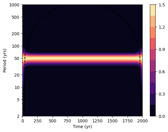
- pyleoclim.utils.wavelet.wwz_basic(ys, ts, freq, tau, c=0.012665147955292222, Neff_threshold=3, nproc=1, detrend=False, sg_kwargs=None, gaussianize=False, standardize=False)[source]
Return the weighted wavelet amplitude (WWA).
The Weighted wavelet Z-transform (WWZ) is based on Morlet wavelet estimation, using least squares minimization to suppress the energy leakage caused by data gaps. WWZ does not rely on interpolation or detrending, and is appropriate for unevenly-spaced datasets. In particular, we use the variant of Kirchner & Neal (2013), in which basis rotations mitigate the numerical instability that occurs in pathological cases with the original algorithm (Foster, 1996). The WWZ method has one adjustable parameter, a decay constant c that balances the time and frequency resolutions of the analysis. This application uses the larger value 1/(8π^2), justified elsewhere (Witt & Schumann, 2005).
No multiprocessing is applied by Default.
- Parameters:
ys (array) – a time series
ts (array) – time axis of the time series
freq (array) – vector of frequency
tau (array) – the evenly-spaced time points, namely the time shift for wavelet analysis
c (float) – the decay constant that determines the analytical resolution of frequency for analysis, the smaller the higher resolution; the default value 1/(8*np.pi**2) is good for most of the wavelet analysis cases
Neff_threshold (int) – the threshold of the number of effective degrees of freedom
nproc (int) – fake argument, just for convenience
detrend (string) – None - the original time series is assumed to have no trend (default); Types of detrending: - “linear” : the result of a linear least-squares fit to y is subtracted from y. - “constant” : only the mean of data is subtracted. - “savitzky-golay” : y is filtered using the Savitzky-Golay filter and the resulting filtered series is subtracted from y. - “emd” : Empirical mode decomposition. The last mode is assumed to be the trend and removed from the series
sg_kwargs (dict) – The parameters for the Savitzky-Golay filter. see pyleoclim.utils.filter.savitzy_golay for details.
gaussianize (bool) – If True, gaussianizes the timeseries
standardize (bool) – If True, standardizes the timeseries
- Returns:
wwa (array) – the weighted wavelet amplitude
phase (array) – the weighted wavelet phase
Neffs (array) – the matrix of effective number of points in the time-scale coordinates
coeff (array) – the wavelet transform coefficients (a0, a1, a2)
References
Foster, G. Wavelets for period analysis of unevenly sampled time series. The Astronomical Journal 112, 1709 (1996).
Witt, A. & Schumann, A. Y. Holocene climate variability on millennial scales recorded in Greenland ice cores. Nonlinear Processes in Geophysics 12, 345–352 (2005).
Kirchner, J. W. and Neal, C. (2013). Universal fractal scaling in stream chemistry and its implications for solute transport and water quality trend detection. Proc Natl Acad Sci USA 110:12213–12218.
See also
pyleoclim.utils.wavelet.wwz_nprocReturns the weighted wavelet amplitude using the original method from Kirchner. Supports multiprocessing
pyleoclim.utils.wavelet.kirchner_basicReturn the weighted wavelet amplitude (WWA) modified by Kirchner. No multiprocessing
pyleoclim.utils.wavelet.kirchner_nprocReturns the weighted wavelet amplitude (WWA) modified by Kirchner. Supports multiprocessing
pyleoclim.utils.wavelet.kirchner_numbaReturn the weighted wavelet amplitude (WWA) modified by Kirchner using Numba package.
pyleoclim.utils.wavelet.kirchner_f2pyReturns the weighted wavelet amplitude (WWA) modified by Kirchner. Uses Fortran. Fastest method but requires a compiler.
pyleoclim.utils.filter.savitzky_golaySmooth (and optionally differentiate) data with a Savitzky-Golay filter.
pyleoclim.utils.tsutils.preprocesspre-processes a times series using Gaussianization and detrending.
pyleoclim.utils.tsutils.detrenddetrending functionalities using 4 possible methods
pyleoclim.utils.tsutils.gaussianizeQuantile maps a 1D array to a Gaussian distribution
pyleoclim.utils.tsutils.standardizeCenters and normalizes a given time series.
- pyleoclim.utils.wavelet.wwz_coherence(y1, t1, y2, t2, smooth_factor=0.25, tau=None, freq=None, freq_method='log', freq_kwargs=None, c=0.012665147955292222, Neff_threshold=3, nproc=8, detrend=False, sg_kwargs=None, verbose=False, method='Kirchner_numba', gaussianize=False, standardize=True)[source]
Returns the wavelet coherence of two time series (WWZ method).
- Parameters:
y1 (array) – first of two time series
y2 (array) – second of the two time series
t1 (array) – time axis of first time series
t2 (array) – time axis of the second time series
tau (array) – the evenly-spaced time points
freq (array) – vector of frequency
c (float) – the decay constant that determines the analytical resolution of frequency for analysis, the smaller the higher resolution; the default value 1/(8*np.pi**2) is good for most of the wavelet analysis cases
Neff_threshold (int) – threshold for the effective number of points
nproc (int) – the number of processes for multiprocessing
detrend (string) –
None: the original time series is assumed to have no trend;
’linear’: a linear least-squares fit to ys is subtracted;
’constant’: the mean of ys is subtracted
’savitzy-golay’: ys is filtered using the Savitzky-Golay filter and the resulting filtered series is subtracted from y.
Empirical mode decomposition. The last mode is assumed to be the trend and removed from the series
sg_kwargs (dict) – The parameters for the Savitzky-Golay filter. see pyleoclim.utils.filter.savitzy_golay for details.
gaussianize (bool) – If True, gaussianizes the timeseries
standardize (bool) – If True, standardizes the timeseries
method (string) –
‘Foster’: the original WWZ method;
’Kirchner’: the method Kirchner adapted from Foster;
’Kirchner_f2py’: the method Kirchner adapted from Foster with f2py
’Kirchner_numba’: Kirchner’s algorithm with Numba support for acceleration (default)
verbose (bool) – If True, print warning messages
smooth_factor (float) – smoothing factor for the WTC (default: 0.25)
- Returns:
res – contains the cross wavelet coherence, cross-wavelet phase, vector of frequency, evenly-spaced time points, AR1 sims, cone of influence
- Return type:
dict
References
Grinsted, A., J. C. Moore, and S. Jevrejeva (2004), Application of the cross wavelet transform and wavelet coherence to geophysical time series, Nonlinear Processes in Geophysics, 11, 561–566.
See also
pyleoclim.utils.wavelet.wwz_basicReturns the weighted wavelet amplitude using the original method from Kirchner. No multiprocessing
pyleoclim.utils.wavelet.wwz_nprocReturns the weighted wavelet amplitude using the original method from Kirchner. Supports multiprocessing
pyleoclim.utils.wavelet.kirchner_basicReturn the weighted wavelet amplitude (WWA) modified by Kirchner. No multiprocessing
pyleoclim.utils.wavelet.kirchner_nprocReturns the weighted wavelet amplitude (WWA) modified by Kirchner. Supports multiprocessing
pyleoclim.utils.wavelet.kirchner_numbaReturn the weighted wavelet amplitude (WWA) modified by Kirchner using Numba package.
pyleoclim.utils.wavelet.kirchner_f2pyReturns the weighted wavelet amplitude (WWA) modified by Kirchner. Uses Fortran. Fastest method but requires a compiler.
pyleoclim.utils.filter.savitzky_golaySmooth (and optionally differentiate) data with a Savitzky-Golay filter.
pyleoclim.utils.wavelet.make_freq_vectorMake frequency vector
pyleoclim.utils.tsutils.detrenddetrending functionalities
pyleoclim.utils.tsutils.gaussianizeQuantile maps a 1D array to a Gaussian distribution
pyleoclim.utils.tsutils.preprocesspre-processes a times series using Gaussianization and detrending.
- pyleoclim.utils.wavelet.wwz_nproc(ys, ts, freq, tau, c=0.012665147955292222, Neff_threshold=3, nproc=8, detrend=False, sg_kwargs=None, gaussianize=False, standardize=False)[source]
Return the weighted wavelet amplitude (WWA).
Original method from Foster (1996). Supports multiprocessing.
- Parameters:
ys (array) – a time series
ts (array) – time axis of the time series
freq (array) – vector of frequency
tau (array) – the evenly-spaced time points, namely the time shift for wavelet analysis
c (float) – the decay constant that determines the analytical resolution of frequency for analysis, the smaller the higher resolution; the default value 1/(8*np.pi**2) is good for most of the wavelet analysis cases
Neff_threshold (int) – the threshold of the number of effective degrees of freedom [default = 3]
nproc (int) – the number of processes for multiprocessing [default = 8]
detrend (string) – False - the original time series is assumed to have no trend; Types of detrending: - “linear” : the result of a linear least-squares fit to y is subtracted from y. - “constant” : only the mean of data is subtracted. - “savitzky-golay” : y is filtered using the Savitzky-Golay filter and the resulting filtered series is subtracted from y. - “emd” : Empirical mode decomposition. The last mode is assumed to be the trend and removed from the series
sg_kwargs (dict) – The parameters for the Savitzky-Golay filter. see pyleoclim.utils.filter.savitzy_golay for details.
gaussianize (bool) – If True, gaussianizes the timeseries
standardize (bool) – If True, standardizes the timeseries
- Returns:
wwa (array) – the weighted wavelet amplitude
phase (array) – the weighted wavelet phase
Neffs (array) – the matrix of effective number of points in the time-scale coordinates
coeff (array) – the wavelet transform coefficients (a0, a1, a2)
See also
pyleoclim.utils.wavelet.wwz_basicweighted wavelet amplitude using the original method from Kirchner. No multiprocessing
pyleoclim.utils.wavelet.kirchner_basicweighted wavelet amplitude (WWA) modified by Kirchner. No multiprocessing
pyleoclim.utils.wavelet.kirchner_nprocweighted wavelet amplitude (WWA) modified by Kirchner. Supports multiprocessing
pyleoclim.utils.wavelet.kirchner_numbaweighted wavelet amplitude (WWA) modified by Kirchner using Numba package.
pyleoclim.utils.wavelet.kirchner_f2pyweighted wavelet amplitude (WWA) modified by Kirchner. Uses Fortran. Fastest method but requires a compiler.
pyleoclim.utils.tsutils.preprocesspre-processes a times series using Gaussianization and detrending.
pyleoclim.utils.filter.savitzky_golaySmooth (and optionally differentiate) data with a Savitzky-Golay filter.
pyleoclim.utils.tsutils.detrenddetrending functionalities
pyleoclim.utils.tsutils.gaussianizeQuantile maps a 1D array to a Gaussian distribution
- pyleoclim.utils.wavelet.xwt(coeff1, coeff2)[source]
Return the cross wavelet transform.
- Parameters:
coeff1 (array) – the first of two sets of wavelet transform coefficients in the form of a1 + a2*1j
coeff2 (array) – the second of two sets of wavelet transform coefficients in the form of a1 + a2*1j
freq (array) – vector of frequency
tau (array) – evenly-spaced time axis (original ttime axis for CWT, time shift for WWZ).
- Returns:
xw_t (array (complex)) – the cross wavelet transform
xw_amplitude (array) – the cross wavelet amplitude
xw_phase (array) – the cross wavelet phase
References
Grinsted, A., Moore, J. C. & Jevrejeva, S. Application of the cross wavelet transform and wavelet coherence to geophysical time series. Nonlin. Processes Geophys. 11, 561–566 (2004).
Tsutils
Utilities to manipulate timeseries - useful for preprocessing prior to analysis
- class pyleoclim.utils.tsutils.EmpiricalModeDecomposition(x, t=None, threshold_1=0.05, threshold_2=0.5, alpha=0.05, ndirs=4, fixe=0, maxiter=2000, fixe_h=0, n_imfs=0, nbsym=2, bivariate_mode='bbox_center')[source]
The EMD class. This class has been adapted from the pyhht package (https://github.com/jaidevd/pyhht/tree/dev) and adapated to work with scipy 0.12.0. See the copyright notice in the emd_utils module.
- decompose()[source]
Decompose the input signal into IMFs.
This function does all the heavy lifting required for sifting, and should ideally be the only public method of this class.
- Returns:
imfs – A matrix containing one IMF per row.
- Return type:
array-like, shape (n_imfs, n_samples)
Examples
>>> from pyhht.visualization import plot_imfs
>>> import numpy as np
>>> t = np.linspace(0, 1, 1000)
>>> modes = np.sin(2 * pi * 5 * t) + np.sin(2 * pi * 10 * t)
>>> x = modes + t
>>> decomposer = EMD(x)
>>> imfs = decomposer.decompose()
- io()[source]
Compute the index of orthoginality, as defined by:
\[\sum_{i,j=1,i\neq j}^{N}\frac{\|C_{i}\overline{C_{j}}\|}{\|x\|^2}\]Where \(C_{i}\) is the \(i\) th IMF.
- Returns:
Index of orthogonality. Lower values are better.
- Return type:
float
- mean_and_amplitude(m)[source]
Compute the mean of the envelopes and the mode amplitudes.
- Parameters:
m (array-like, shape (n_samples,)) – The input array or an itermediate value of the sifting process.
- Returns:
A tuple containing the mean of the envelopes, the number of extrema, the number of zero crosssing and the estimate of the amplitude of themode.
- Return type:
tuple
- pyleoclim.utils.tsutils.annualize(ys, ts)[source]
Annualize a time series whose time resolution is finer than 1 year
- Parameters:
ys (array) – A time series, NaNs allowed
ts (array) – The time axis of the time series, NaNs allowed
- Returns:
ys_ann (array) – the annualized time series
year_int (array) – The time axis of the annualized time series
- pyleoclim.utils.tsutils.calculate_distances(ys, n_neighbors=None, NN_kwargs=None)[source]
Uses the scikit-learn unsupervised learner for implementing neighbor searches and calculate the distance between a point and its nearest neighbors to estimate epsilon for DBSCAN.
- Parameters:
ys (numpy.array) – the y-values for the timeseries
n_neighbors (int, optional) – Number of neighbors to use by default for kneighbors queries. The default is None.
NN_kwargs (dict, optional) – Other arguments for sklearn.neighbors.NearestNeighbors. The default is None. See: https://scikit-learn.org/stable/modules/generated/sklearn.neighbors.NearestNeighbors.html#sklearn.neighbors.NearestNeighbors
- Returns:
min_eps (int) – Minimum value for epsilon.
max_eps (int) – Maximum value for epsilon.
- pyleoclim.utils.tsutils.center(y, axis=0)[source]
Centers array y (i.e. removes the sample mean)
- Parameters:
y (array) – Vector of (real) numbers as a time series, NaNs allowed
axis (int or None) – Axis along which to operate, if None, compute over the whole array
- Returns:
yc (array) – The centered time series, yc = (y - ybar), NaNs allowed
ybar (real) – The sampled mean of the original time series, y
References
Tapio Schneider’s MATLAB code: https://github.com/tapios/RegEM/blob/master/center.m
- pyleoclim.utils.tsutils.custom_year_averages(data: Series, start_month: int, end_month: int, years: Optional[Union[int, list, range]] = None) Series[source]
Compute weighted averages over custom year periods that may straddle calendar years.
- Parameters:
data (pd.Series) – Time series data with DatetimeIndex. Can be daily or monthly frequency.
start_month (int) – Starting month of the custom year (1-12).
end_month (int) – Ending month of the custom year (1-12).
years (int, list, range, or None) – Year(s) for which to compute averages. If None, computes for all available years. For straddling periods (e.g., Apr-Mar), year refers to the year of the end month.
- Returns:
Series index by year, with weighted averages as values.
- Return type:
pd.Series
Examples
import pandas as pd
import numpy as np
import pyleoclim.utils.tsutils as ut

# Create sample monthly data
dates = pd.date_range('2020-01-01', '2023-12-31', freq='ME')
values = np.arange(len(dates))  # Sequential values for clarity
ts = pd.Series(values, index=dates, name='monthly_values')

# Example 1: Single year (int)
# Compute Jan-Mar average for 2021 only
avg_single = ut.custom_year_averages(ts, 1, 3, years=2021)
print("Single year (2021):")
print(avg_single)
print()

# Example 2: List of specific years
# Compute Apr-Mar averages for selected years
avg_list = ut.custom_year_averages(ts, 4, 3, years=[2021, 2023])
print("Specific years [2021, 2023]:")
print(avg_list)
print()

# Example 3: Range of years
# Compute Oct-Sep averages for consecutive years
avg_range = ut.custom_year_averages(ts, 10, 9, years=range(2021, 2024))
print("Range of years (2021-2023):")
print(avg_range)
print()

# Example 4: All available years (None - default)
# Compute Jan-Dec averages for all years in data
avg_all = ut.custom_year_averages(ts, 1, 12, years=None)
print("All available years (None):")
print(avg_all)
print()

# Example 5: Straddling periods with different year specifications
# Apr-Mar periods: year refers to the March year
avg_straddle = ut.custom_year_averages(ts, 4, 3, years=range(2021, 2024))
print("Straddling periods (Apr-Mar), years 2021-2023:")
print(avg_straddle)
Single year (2021):
2021    13.0
Name: monthly_values, dtype: float64

Specific years [2021, 2023]:
2021     8.5
2023    32.5
Name: monthly_values, dtype: float64

Range of years (2021-2023):
2021    14.5
2022    26.5
2023    38.5
Name: monthly_values, dtype: float64

All available years (None):
2020     5.5
2021    17.5
2022    29.5
2023    41.5
Name: monthly_values, dtype: float64

Straddling periods (Apr-Mar), years 2021-2023:
2021     8.5
2022    20.5
2023    32.5
Name: monthly_values, dtype: float64
# Daily data example with uneven spacing
daily_dates = pd.to_datetime([
    '2021-01-01', '2021-01-05', '2021-01-20',
    '2021-02-01', '2021-02-15', '2021-02-28',
    '2021-03-05', '2021-03-25', '2021-03-31'
])
daily_values = [10, 15, 20, 25, 30, 35, 40, 45, 50]
daily_ts = pd.Series(daily_values, index=daily_dates, name='daily_data')

# Compute weighted average (accounts for uneven spacing)
daily_avg = ut.custom_year_averages(daily_ts, 1, 3, years=2021)
print("Daily data with uneven spacing (Jan-Mar 2021):")
print(f"Weighted average: {daily_avg.iloc[0]:.2f}")
print(f"Simple mean: {daily_ts.mean():.2f}")
print("(Note: weighted average accounts for time intervals between observations)")
Daily data with uneven spacing (Jan-Mar 2021):
Weighted average: 30.48
Simple mean: 30.00
(Note: weighted average accounts for time intervals between observations)
- pyleoclim.utils.tsutils.detect_outliers_DBSCAN(ys, nbr_clusters=None, eps=None, min_samples=None, n_neighbors=None, metric='euclidean', NN_kwargs=None, DBSCAN_kwargs=None)[source]
Uses the unsupervised learning DBSCAN algorithm to identify outliers in timeseries data. The algorithm uses the silhouette score calculated over a range of epsilon and minimum sample values to determine the best clustering. In this case, we take the largest silhouette score (as close to 1 as possible).
The DBSCAN implementation used here is from scikit-learn: https://scikit-learn.org/stable/modules/generated/sklearn.cluster.DBSCAN.html
The Silhouette Coefficient is calculated using the mean intra-cluster distance (a) and the mean nearest-cluster distance (b) for each sample. The best value is 1 and the worst value is -1. Values near 0 indicate overlapping clusters. Negative values generally indicate that a sample has been assigned to the wrong cluster, as a different cluster is more similar. For additional details, see: https://scikit-learn.org/stable/modules/generated/sklearn.metrics.silhouette_score.html
- Parameters:
ys (numpy.array) – The y-values for the timeseries data.
nbr_clusters (int, optional) – Number of clusters. Note that the DBSCAN algorithm calculates the number of clusters automatically. This paramater affects the optimization over the silhouette score. The default is None.
eps (float or list, optional) – epsilon. The default is None, which allows the algorithm to optimize for the best value of eps, using the silhouette score as the optimization criterion. The maximum distance between two samples for one to be considered as in the neighborhood of the other. This is not a maximum bound on the distances of points within a cluster. This is the most important DBSCAN parameter to choose appropriately for your data set and distance function.
min_samples (int or list, optional) – The number of samples (or total weight) in a neighborhood for a point to be considered as a core point. This includes the point itself.. The default is None and optimized using the silhouette score
n_neighbors (int, optional) – Number of neighbors to use by default for kneighbors queries, which can be used to calculate a range of plausible eps values. The default is None.
metric (str, optional) – The metric to use when calculating distance between instances in a feature array. The default is ‘euclidean’. See https://scikit-learn.org/stable/modules/generated/sklearn.cluster.DBSCAN.html for alternative values.
NN_kwargs (dict, optional) – Other arguments for sklearn.neighbors.NearestNeighbors. The default is None. See: https://scikit-learn.org/stable/modules/generated/sklearn.neighbors.NearestNeighbors.html#sklearn.neighbors.NearestNeighbors
DBSCAN_kwargs (dict, optional) – Other arguments for sklearn.cluster.DBSCAN. The default is None. See: https://scikit-learn.org/stable/modules/generated/sklearn.cluster.DBSCAN.html
- Returns:
indices (list) – list of indices that are considered outliers.
res (pandas.DataFrame) – Results of the clustering analysis. Contains information about eps value, min_samples value, number of clusters, the silhouette score, the indices of the outliers for each combination, and the cluster assignment for each point.
- pyleoclim.utils.tsutils.detect_outliers_kmeans(ys, nbr_clusters=None, max_cluster=10, threshold=3, LOF=False, n_frac=0.9, contamination='auto', kmeans_kwargs=None)[source]
Outlier detection using the unsupervised alogrithm kmeans. The algorithm runs through various number of clusters and optimizes based on the silhouette score.
KMeans implementation: https://scikit-learn.org/stable/modules/generated/sklearn.cluster.KMeans.html
The Silhouette Coefficient is calculated using the mean intra-cluster distance (a) and the mean nearest-cluster distance (b) for each sample. The best value is 1 and the worst value is -1. Values near 0 indicate overlapping clusters. Negative values generally indicate that a sample has been assigned to the wrong cluster, as a different cluster is more similar. For additional details, see: https://scikit-learn.org/stable/modules/generated/sklearn.metrics.silhouette_score.html
Outliers are identified based on their distance from the clusters. This can be done in two ways: (1) by using a threshold that corresponds to the Euclidean distance from the centroid and (2) using the Local Outlier Function (https://scikit-learn.org/stable/auto_examples/neighbors/plot_lof_outlier_detection.html)
- Parameters:
ys (numpy.array) – The y-values for the timeseries data
nbr_clusters (int or list, optional) – A user number of clusters to considered. The default is None.
max_cluster (int, optional) – The maximum number of clusters to consider in the optimization based on the Silhouette Score. The default is 10.
threshold (int, optional) – The algorithm uses the euclidean distance for each point in the cluster to identify the outliers. This parameter sets the threshold on the euclidean distance to define an outlier. The default is 3.
LOF (bool, optional) – By default, detect_outliers_kmeans uses euclidean distance for outlier detection. Set LOF to True to use LocalOutlierFactor for outlier detection.
n_frac (float, optional) – The percentage of the time series length (the length, representing number of points) to be used to set the n_neighbors parameter for the LOF function in scikit-learn. We recommend using at least 50% (n_frac=0.5) of the timeseries. You cannot use 100% (n_frac!=1)
contamination (('auto', float), optional) – Same as LOF parameter from scikit-learn. We recommend using the default mode of auto. See: https://scikit-learn.org/stable/modules/generated/sklearn.neighbors.LocalOutlierFactor.html for details.
kmeans_kwargs (dict, optional) – Other parameters for the kmeans function. See: https://scikit-learn.org/stable/modules/generated/sklearn.cluster.KMeans.html for details. The default is None.
- Returns:
indices (list) – list of indices that are considered outliers.
res (pandas.DataFrame) – Results of the clustering analysis. Contains information about number of clusters, the silhouette score, the indices of the outliers for each combination, and the cluster assignment for each point.
- pyleoclim.utils.tsutils.detrend(y, x=None, method='emd', n=1, preserve_mean=False, sg_kwargs=None)[source]
Detrend a timeseries according to four methods
Detrending methods include: “linear”, “constant”, using a low-pass Savitzky-Golay filter, and Empirical Mode Decomposition (default). Linear and constant methods use scipy.signal.detrend., EMD uses pyhht.emd.EMD.
- Parameters:
y (array) – The series to be detrended.
x (array) – Abscissa for array y. Necessary for use with the Savitzky-Golay method, since the series should be evenly spaced.
method (str) –
The type of detrending:
”linear”: the result of a linear least-squares fit to y is subtracted from y.
”constant”: only the mean of data is subtracted.
”savitzky-golay”, y is filtered using the Savitzky-Golay filters and the resulting filtered series is subtracted from y.
”emd” (default): Empirical mode decomposition. The last mode is assumed to be the trend and removed from the series
n (int) – Works only if method == ‘emd’. The number of smoothest modes to remove.
preserve_mean (boolean) – flag to indicate whether the mean of the series should be preserved despite the detrending
sg_kwargs (dict) – The parameters for the Savitzky-Golay filters.
- Returns:
ys (array) – The detrended version of y.
trend (array) – The removed trend. Only non-empty for EMD and Savitzy-Golay methods, since SciPy detrending does not retain the trends
See also
pyleoclim.utils.filter.savitzky_golayFiltering using Savitzy-Golay
pyleoclim.utils.tsutils.preprocesspre-processes a times series using standardization and detrending.
- pyleoclim.utils.tsutils.eff_sample_size(y, detrend_flag=False)[source]
Effective Sample Size of timeseries y
- Parameters:
y (float) – 1d array
detrend_flag (boolean) – if True (default), detrends y before estimation.
- Returns:
neff – The effective sample size
- Return type:
float
References
Thiébaux HJ and Zwiers FW, 1984: The interpretation and estimation of effective sample sizes. Journal of Climate and Applied Meteorology 23: 800–811.
- pyleoclim.utils.tsutils.gauss(ys)
Maps a 1D array to a Gaussian distribution using the inverse Rosenblatt transform
The resulting array is mapped to a standard normal distribution, and therefore has zero mean and unit standard deviation. Using gaussianize() obviates the need for standardize().
- Parameters:
ys (1D Array) – e.g. a timeseries
- Returns:
yg – Gaussianized values of ys.
- Return type:
1D Array
References
- van Albada, S., and P. Robinson (2007), Transformation of arbitrary
distributions to the normal distribution with application to EEG test-retest reliability, Journal of Neuroscience Methods, 161(2), 205 - 211, doi:10.1016/j.jneumeth.2006.11.004.
See also
pyleoclim.utils.tsutils.standardizeCenters and normalizes a time series
- pyleoclim.utils.tsutils.gaussianize(ys)[source]
Maps a 1D array to a Gaussian distribution using the inverse Rosenblatt transform
The resulting array is mapped to a standard normal distribution, and therefore has zero mean and unit standard deviation. Using gaussianize() obviates the need for standardize().
- Parameters:
ys (1D Array) – e.g. a timeseries
- Returns:
yg – Gaussianized values of ys.
- Return type:
1D Array
References
- van Albada, S., and P. Robinson (2007), Transformation of arbitrary
distributions to the normal distribution with application to EEG test-retest reliability, Journal of Neuroscience Methods, 161(2), 205 - 211, doi:10.1016/j.jneumeth.2006.11.004.
See also
pyleoclim.utils.tsutils.standardizeCenters and normalizes a time series
- pyleoclim.utils.tsutils.gkernel(t, y, h=None, step=None, start=None, stop=None, step_style=None, evenly_spaced=False, bin_edges=None, time_axis=None, no_nans=True)[source]
Coarsen time resolution using a Gaussian kernel
The behavior of bins, as defined either by start, stop and step (or step_style) or by the bins argument, is to have all bins except the last one be half open. That is if bins are defined as bins = [1,2,3,4], bins will be [1,2), [2,3), [3,4]. This is the default behaviour of our binning functionality (upon which this function is based).
- Parameters:
t (1d array) – the original time axis
y (1d array) – values on the original time axis
h (float) – kernel e-folding scale. Default value is None, in which case the median time step will be used. If the median time step results in a series with nan values, the maximum time step will be used. Note that if this variable is too small, this method may return nan values in parts of the series.
step (float) – The interpolation step. Default is max spacing between consecutive points.
start (float) – where/when to start the interpolation. Default is min(t).
stop (float) – where/when to stop the interpolation. Default is max(t).
step_style (str) – step style to be applied from ‘increments’ [default = ‘max’]
evenly_spaced ({True,False}) – Makes the series evenly-spaced. This option is ignored if bins are passed. This option is being deprecated, no_nans should be used instead.
bin_edges (array) – The right hand edge of bins to use for binning. E.g. if bins = [1,2,3,4], bins will be [1,2), [2,3), [3,4]. Same behavior as scipy.stats.binned_statistic Start, stop, step, and step_style will be ignored if this is passed.
time_axis (np.ndarray) – The time axis to use for binning. If passed, bin_edges will be set as the midpoints between times. The first time will be used as the left most edge, the last time will be used as the right most edge. Start, stop, bin_size, and step_style will be ignored if this is passed.
no_nans (bool; {True,False}) – Sets the step_style to max, ensuring that the resulting series contains no empty values (nans). Default is True.
- Returns:
tc (1d array) – the coarse-grained time axis
yc (1d array) – The coarse-grained time series
Notes
start, stop, step, and step_style are interpreted as defining the bin_edges for this function. This differs from the interp interpretation, which uses these to define the time axis over which interpolation is applied. For gkernel, the time axis will be specified as the midpoints between bin_edges, unless time_axis is explicitly passed.
References
Rehfeld, K., Marwan, N., Heitzig, J., and Kurths, J.: Comparison of correlation analysis techniques for irregularly sampled time series, Nonlin. Processes Geophys., 18, 389–404, doi:10.5194/npg-18-389-2011, 2011.
See also
pyleoclim.utils.tsutils.incrementsEstablishes the increments of a numerical array
pyleoclim.utils.tsutils.make_even_axisCreate an even time axis
pyleoclim.utils.tsutils.binBin the values
pyleoclim.utils.tsutils.interpInterpolate y onto a new x-axis
Examples
There are several ways to specify the way coarsening is done via this function. Within these there is a hierarchy which we demonstrate below.
Top priority is given to bin_edges if it is not None. All other arguments will be ignored (except for x and y). The resulting time axis will be comprised of the midpoints between bin edges.
import numpy as np
import pyleoclim as pyleo

x = np.array([1,2,3,5,8,12,20])
y = np.ones(len(x))
xc,yc = pyleo.utils.tsutils.gkernel(x,y,bin_edges=[1,4,8,12,16,20])
xc
array([ 2.5, 6. , 10. , 14. , 18. ])
Next, priority will go to time_axis if it is passed. In this case, bin edges will be taken as the midpoints between time axis points. The first and last time point will be used as the left most and right most bin edges.
x = np.array([1,2,3,5,8,12,20])
y = np.ones(len(x))
xc,yc = pyleo.utils.tsutils.gkernel(x,y,time_axis=[1,4,8,12,16,20])
xc
array([ 1, 4, 8, 12, 16, 20])
If time_axis is None, step will be considered, overriding step_style if it is passed. start and stop will be generated using defaults if not passed.
x = np.array([1,2,3,5,8,12,20])
y = np.ones(len(x))
xc,yc = pyleo.utils.tsutils.gkernel(x,y,step=2)
xc
array([ 2., 4., 6., 8., 10., 12., 14., 16., 18.])
If both time_axis and step are None but step_style is specified, the step will be generated using the prescribed step_style.
x = np.array([1,2,3,5,8,12,20])
y = np.ones(len(x))
xc,yc = pyleo.utils.tsutils.gkernel(x,y,step_style='max')
xc
array([ 5., 13.])
If none of these are specified, the mean spacing will be used.
x = np.array([1,2,3,5,8,12,20])
y = np.ones(len(x))
xc,yc = pyleo.utils.tsutils.gkernel(x,y)
xc
array([ 5., 13.])
- pyleoclim.utils.tsutils.increments(x, step_style='median')[source]
Establishes the increments of a numerical array: start, stop, and representative step.
- Parameters:
x (array) –
step_style (str) –
Method to obtain a representative step if x is not evenly spaced. Valid entries: ‘median’ [default], ‘mean’, ‘mode’ or ‘max’ The mode is the most frequent entry in a dataset, and may be a good choice if the timeseries is nearly equally spaced but for a few gaps.
Max is a conservative choice, appropriate for binning methods and Gaussian kernel coarse-graining
- Returns:
start (float) – min(x)
stop (float) – max(x)
step (float) – The representative spacing between consecutive values, computed as above
See also
pyleoclim.utils.tsutils.binBin the values
pyleoclim.utils.tsutils.gkernelCoarsen time resolution using a Gaussian kernel
- pyleoclim.utils.tsutils.interp(x, y, interp_type='linear', step=None, start=None, stop=None, step_style=None, time_axis=None, **kwargs)[source]
Interpolate y onto a new x-axis
Largely a wrapper for scipy.interpolate.interp1d.
- Parameters:
x (array) – The x-axis
y (array) – The y-axis
interp_type (str) – Options include: ‘linear’, ‘nearest’, ‘zero’, ‘slinear’, ‘quadratic’, ‘cubic’, ‘previous’, ‘next’ where ‘zero’, ‘slinear’, ‘quadratic’ and ‘cubic’ refer to a spline interpolation of zeroth, first, second or third order; ‘previous’ and ‘next’ simply return the previous or next value of the point) or as an integer specifying the order of the spline interpolator to use. Default is ‘linear’.
step (float) – The interpolation step. Default is mean spacing between consecutive points. Step_style will be ignored if this is passed.
start (float) – Where/when to start the interpolation. Default is the minimum.
stop (float) – Where/when to stop the interpolation. Default is the maximum.
step_style (str; {'min','mean','median','max'}) – Step style to use when determining the size of the interval between points. Default is None.
time_axis (np.ndarray) – Time axis onto which the series will be interpolated. Start, stop, step, and step_style will be ignored if this is passed
kwargs (kwargs) – Aguments specific to interpolate.interp1D. If getting an error about extrapolation, you can use the arguments bound_errors=False and fill_value=”extrapolate” to allow for extrapolation.
- Returns:
xi (array) – The interpolated x-axis
yi (array) – The interpolated y values
Notes
start, stop, step and step_styl`e pertain to the creation of the time axis over which interpolation will be conducted. This differs from the way that the functions `bin and gkernel interpret these arguments, which is as defining the bin_edges parameter used in those functions.
See also
pyleoclim.utils.tsutils.incrementsEstablishes the increments of a numerical array
pyleoclim.utils.tsutils.make_even_axisMakes an evenly spaced time axis
pyleoclim.utils.tsutils.binBin the values
pyleoclim.utils.tsutils.gkernelCoarsen time resolution using a Gaussian kernel
Examples
There are several ways to specifiy a time axis for interpolation. Within these there is a hierarchy which we demonstrate below.
Top priority will always go to time_axis if it is passed. All other arguments will be overwritten (except for x,y, and interp_type).
import numpy as np
import pyleoclim as pyleo

x = np.array([1,2,3,5,8,12,20])
y = np.ones(len(x))
xi,yi = pyleo.utils.tsutils.interp(x,y,time_axis=[1,4,8,12,16])
xi
array([ 1, 4, 8, 12, 16])
If time_axis is None, step will be considered, overriding step_style if it is passed. `start and stop will be generated using defaults if not passed.
x = np.array([1,2,3,5,8,12,20])
y = np.ones(len(x))
xi,yi = pyleo.utils.tsutils.interp(x,y,step=2)
xi
array([ 1., 3., 5., 7., 9., 11., 13., 15., 17., 19.])
If both time_axis and step are None but step_style is specified, the step will be generated using the prescribed step_style.
x = np.array([1,2,3,5,8,12,20])
y = np.ones(len(x))
xi,yi = pyleo.utils.tsutils.interp(x,y,step_style='max')
xi
array([ 1., 9., 17.])
If none of these are specified, the mean spacing will be used.
x = np.array([1,2,3,5,8,12,20])
y = np.ones(len(x))
xi,yi = pyleo.utils.tsutils.interp(x,y)
xi
array([ 1.        ,  4.16666667,  7.33333333, 10.5       , 13.66666667,
       16.83333333, 20.        ])
- pyleoclim.utils.tsutils.make_even_axis(x=None, start=None, stop=None, step=None, step_style=None, no_nans=False)[source]
Create a uniform time axis for binning/interpolating
- Parameters:
x (np.ndarray) – Uneven time axis upon which to base the uniform time axis.
start (float) – Where to start the axis. Default is the first value of the passed time axis.
stop (float) – Where to stop the axis. Default is the last of value of the passed time axis.
step (float) – The step size to use for the axis. Must be greater than 0.
step_style (str; {}) – Step style to use when defining the step size. Will be overridden by step if it is passed.
no_nans (bool: {True,False}) – Whether or not to allow nans. When True, will set step style to ‘max’. Will be overridden by step_style or step if they are passed. Default is False.
------- –
time_axis (np.ndarray) – An evenly spaced time axis.
- pyleoclim.utils.tsutils.phaseran(y, nsurr)[source]
Phase randomization of a time series y, of even or odd length.
Closely follows this strategy: https://stackoverflow.com/q/39543002
- Parameters:
y (array, length nt) – Signal to be scrambled
nsurr (int) – is the number of image block surrogates that you want to generate.
- Returns:
ysurr – Array of y surrogates
- Return type:
array nt x nsurr
See also
pyleoclim.utils.correlation.fdrDetermine significance based on the false discovery rate
References
Prichard, D., Theiler, J. Generating Surrogate Data for Time Series with Several Simultaneously Measured Variables (1994) Physical Review Letters, Vol 73, Number 7
- pyleoclim.utils.tsutils.preprocess(ys, ts, detrend=False, sg_kwargs=None, gaussianize=False, standardize=True)[source]
Return the processed time series using detrend and standardization.
- Parameters:
ys (array) – a time series
ts (array) – The time axis for the timeseries. Necessary for use with the Savitzky-Golay filters method since the series should be evenly spaced.
detrend (string) – ‘none’/False/None - no detrending will be applied; ‘emd’ - the last mode is assumed to be the trend and removed from the series ‘linear’ - a linear least-squares fit to ys is subtracted; ‘constant’ - the mean of ys is subtracted ‘savitzy-golay’ - ys is filtered using the Savitzky-Golay filter and the resulting filtered series is subtracted.
sg_kwargs (dict) – The parameters for the Savitzky-Golay filter.
gaussianize (bool) – If True, gaussianizes the timeseries
standardize (bool) – If True, standardizes the timeseries
- Returns:
res – the processed time series
- Return type:
array
See also
pyleoclim.utils.tsutils.detrendDetrend a timeseries according to four methods
pyleoclim.utils.filter.savitzy_golayFiltering using Savitzy-Golay method
pyleoclim.utils.tsutils.standardizeCenters and normalizes a given time series
pyleoclim.utils.tsutils.gaussianizeQuantile maps a matrix to a Gaussian distribution
- pyleoclim.utils.tsutils.remove_outliers(ts, ys, indices)[source]
Remove the outliers from timeseries data
- Parameters:
ts (numpy.array) – The time axis for the timeseries data.
ys (numpy.array) – The y-values for the timeseries data.
indices (numpy.array) – The indices of the outliers to be removed.
- Returns:
ys (numpy.array) – The time axis for the timeseries data after outliers removal
ts (numpy.array) – The y-values for the timeseries data after outliers removal
- pyleoclim.utils.tsutils.simple_stats(y, axis=None)[source]
Computes simple statistics
Computes the mean, median, min, max, standard deviation, and interquartile range of a numpy array y, ignoring NaNs.
- Parameters:
y (array) – A Numpy array
axis (int, tuple of ints) – Axis or Axes along which the means are computed, the default is to compute the mean of the flattened array. If a tuple of ints, performed over multiple axes
- Returns:
mean (float) – mean of y, ignoring NaNs
median (float) – median of y, ignoring NaNs
min_ (float) – mininum value in y, ignoring NaNs
max_ (float) – max value in y, ignoring NaNs
std (float) – standard deviation of y, ignoring NaNs
IQR (float) – Interquartile range of y along specified axis, ignoring NaNs
- pyleoclim.utils.tsutils.standardize(x, scale=1, axis=0, ddof=0, eps=0.001)[source]
Centers and normalizes a time series. Constant or nearly constant time series not rescaled.
- Parameters:
x (array) – vector of (real) numbers as a time series, NaNs allowed
scale (real) – A scale factor used to scale a record to a match a given variance
axis (int or None) – axis along which to operate, if None, compute over the whole array
ddof (int) – degress of freedom correction in the calculation of the standard deviation
eps (real) – a threshold to determine if the standard deviation is too close to zero
- Returns:
z (array) – The standardized time series (z-score), Z = (X - E[X])/std(X)*scale, NaNs allowed
mu (real) – The mean of the original time series, E[X]
sig (real) – The standard deviation of the original time series, std[X]
References
Tapio Schneider’s MATLAB code: https://github.com/tapios/RegEM/blob/master/standardize.m
The zscore function in SciPy: https://docs.scipy.org/doc/scipy/reference/generated/scipy.stats.zscore.html
See also
pyleoclim.utils.tsutils.preprocesspre-processes a times series using standardization and detrending.
- pyleoclim.utils.tsutils.std(x, scale=1, axis=0, ddof=0, eps=0.001)
Centers and normalizes a time series. Constant or nearly constant time series not rescaled.
- Parameters:
x (array) – vector of (real) numbers as a time series, NaNs allowed
scale (real) – A scale factor used to scale a record to a match a given variance
axis (int or None) – axis along which to operate, if None, compute over the whole array
ddof (int) – degress of freedom correction in the calculation of the standard deviation
eps (real) – a threshold to determine if the standard deviation is too close to zero
- Returns:
z (array) – The standardized time series (z-score), Z = (X - E[X])/std(X)*scale, NaNs allowed
mu (real) – The mean of the original time series, E[X]
sig (real) – The standard deviation of the original time series, std[X]
References
Tapio Schneider’s MATLAB code: https://github.com/tapios/RegEM/blob/master/standardize.m
The zscore function in SciPy: https://docs.scipy.org/doc/scipy/reference/generated/scipy.stats.zscore.html
See also
pyleoclim.utils.tsutils.preprocesspre-processes a times series using standardization and detrending.
- pyleoclim.utils.tsutils.ts2segments(ys, ts, factor=10)[source]
Chop a time series into several segments based on gap detection.
- The rule of gap detection is very simple:
we define the intervals between time points as dts, then if dts[i] is larger than factor * dts[i-1], we think that the change of dts (or the gradient) is too large, and we regard it as a breaking point and chop the time series into two segments here
- Parameters:
ys (array) – A time series, NaNs allowed
ts (array) – The time points
factor (float) – The factor that adjusts the threshold for gap detection
- Returns:
seg_ys (list) – A list of several segments with potentially different lengths
seg_ts (list) – A list of the time axis of the several segments
n_segs (int) – The number of segments
Tsbase
Basic functionalities to clean timeseries data prior to analysis
- pyleoclim.utils.tsbase.clean_ts(ys, ts, verbose=False)[source]
Cleaning the timeseries
Delete the NaNs in the time series and sort it with time axis ascending, duplicate timestamps will be reduced by averaging the values.
- Parameters:
ys (array) – A time series, NaNs allowed
ts (array) – The time axis of the time series, NaNs allowed
verbose (bool) – If True, will print a warning message
- Returns:
ys (array) – The time series without nans
ts (array) – The time axis of the time series without nans
See also
pyleoclim.utils.tsbase.dropnaDrop NaN values
pyleoclim.utils.tsbase.sort_tsSort timeseries
pyleoclim.utils.tsbase.reduce_duplicated_timestampsConsolidate duplicated timestamps
- pyleoclim.utils.tsbase.convert_datetime_index_to_time(datetime_index, time_unit, time_name)[source]
Convert a Pandas DatetimeIndex into a numpy array of floats.
The general formula is:
datetime_index = datum +/- time*10**exponent
where we assume
timeto use the Gregorian calendar. If dealing with other calendars, then conversions need to happen before reaching pyleoclim.- Parameters:
datetime_index (pd.DatetimeIndex) – Index to covert to floats
time_unit (str) – Time unit indicates the major unit of time. Examples: annum (yr), kiloyear (ka, ky), milayear (ma, my), gigayear (ga, gy)
time_name (str) – If ‘age’, direction is always ‘retrograde’.
- Return type:
np.array((float,)) of converted times
Examples
from pyleoclim.utils.tsbase import convert_datetime_index_to_time
import pandas as pd
import numpy as np

time_unit = 'ga'
time_name = None
dti = pd.date_range("2018-01-01", periods=5, freq="YE", unit='s')
df = pd.DataFrame(np.array(range(5)), index=dti)
time = convert_datetime_index_to_time(
            df.index,
            time_unit,
            time_name=time_name,
            )
print(np.array(time))
[-6.89980514e-08 -6.99973883e-08 -7.09994631e-08 -7.19987999e-08
 -7.29981368e-08]
- pyleoclim.utils.tsbase.disambiguate_time_metadata(time_unit)[source]
Infer time_name and time_unit from (possibly ambiguous) time units as commonly provided in the field.
- Parameters:
time_unit (str) – time units, preferaby something like “kyr BP” or ‘year C.E.’. Otherwise, wild guesses will be attempted to decipher your meaning.
- Returns:
time_name (str) – Name of the time vector (e.g., ‘Time’,’Age’). Possibly None if no guess could be made
time_unit (str) – Updated units for the time vector (e.g., ‘ky BP’).
- pyleoclim.utils.tsbase.is_evenly_spaced(x, tol=0.0001)[source]
Check if an axis x is evenly spaced, within a given tolerance
- Parameters:
x (array) –
tol (float64) – Numerical tolerance for the relative difference
- Returns:
check – True - evenly spaced; False - unevenly spaced.
- Return type:
bool
- pyleoclim.utils.tsbase.overlap(t1, t2)[source]
Computes length of overlap between two time axes. Negative numbers indicate a lack of overlap. Note that this does not count the number of overlapping time stamps ; it merely checks that the two axes have a nonzero intersection on the real line. The amount of points in common depends on how densely sampled these axes are.
- Parameters:
t1 (array) – time axis 1
t2 (array) – time axis 2 (though order doesn’t matter)
- Returns:
L
- Return type:
length of overlap
- pyleoclim.utils.tsbase.reduce_duplicated_timestamps(ys, ts, verbose=False)[source]
Consolidate duplicated timestamps
Reduce duplicated timestamps in a timeseries by averaging the values
- Parameters:
ys (array) – Dependent variable
ts (array) – Independent variable
verbose (bool) – If True, will print a warning message
- Returns:
ys (array) – Dependent variable
ts (array) – Independent variable, with duplicated timestamps reduced by averaging the values
- pyleoclim.utils.tsbase.sort_ts(ys, ts, ascending=True, verbose=False)[source]
Sort timeseries
- Parameters:
ys (array) – Dependent variable
ts (array) – Independent variable
verbose (bool) – If True, will print a warning message
- Returns:
ys (array) – Dependent variable
ts (array) – Independent variable, sorted in ascending order
- pyleoclim.utils.tsbase.time_to_datetime(time, datum=0, exponent=0, direction='prograde', unit='s')[source]
Converts a vector of time values to a pandas datetime object
The general formula is:
datetime_index = datum +/- time*10**exponent
where we assume
timeto use the Gregorian calendar. If dealing with other calendars, then conversions need to happen before reaching pyleoclim.- Parameters:
time (array-like) – the time axis to be converted
datum (int, optional) – origin point for the time scale. The default is 0.
exponent (int, optional) – Base-10 exponent for year multiplier. Dates in kyr should use 3, dates in Myr should use 6, etc. The default is 0.
direction (str, optional) – Direction of time flow, ‘prograde’ [default] or ‘retrograde’.
unit (str, optional) – Units of the datetime. Default is ‘s’, corresponding to seconds. Only change if you have an excellent reason to use finer resolution!
- Return type:
index, a datetime64[unit] object
- pyleoclim.utils.tsbase.time_unit_to_datum_exp_dir(time_unit, time_name=None, verbose=False)[source]
Convert time unit (yr, ka, ma, etc) to a datum, exponent, direction triplet. Based on the time_unit (and optionally, the time_name) the datum (year zero), exponent (10^x year units), and direction (prograde/retrograde) can be inferred. A verbose option is included here for users who want to confirm the resulting inference.
- Parameters:
time_unit (str) – Time unit indicates the major unit of time. Examples: annum (yr), kiloyear (ka, ky), milayear (ma, my), gigayear (ga, gy)
time_name (str) – (Optional) If ‘age’, direction is always ‘retrograde’. Defaults to None, which is effectively unused.
verbose (bool) – (Optional) If True, includes a print statement explaining the conversion.
- Returns:
datum (int, optional) – origin point for the time scale.
exponent (int, optional) – Base-10 exponent for year multiplier. Dates in kyr should use 3, dates in Myr should use 6, etc.
direction (str) – Direction of time flow, ‘prograde’ or ‘retrograde’.
Examples
from pyleoclim.utils.tsbase import time_unit_to_datum_exp_dir

(datum, exponent, direction) = time_unit_to_datum_exp_dir(time_unit)
(datum, exponent, direction)
(1950, 9, 'retrograde')
Lipdutils
Utilities to manipulate LiPD files and automate data transformation whenever possible. These functions are used throughout Pyleoclim but are not meant for direct interaction by users. Also handles integration with the LinkedEarth wiki and the LinkedEarth Ontology.
- pyleoclim.utils.lipdutils.LipdToOntology(archiveType)[source]
standardize archiveType
Transform the archiveType from their LiPD name to their ontology counterpart
- Parameters:
archiveType (string) – name of the archiveType from the LiPD file
- Returns:
archiveType – archiveType according to the ontology
- Return type:
string
- pyleoclim.utils.lipdutils.PLOT_DEFAULT = {'Borehole': ['#FFD600', 's'], 'Coral': ['#FF8B00', 'v'], 'Documents': ['#f8d568', 'p'], 'FluvialSediment': ['#5fa2ce', 'o'], 'GlacierIce': ['deepskyblue', '*'], 'GroundIce': ['slategray', '*'], 'Hybrid': ['#808000', 'H'], 'Instrumental': ['#B07AA1', 'D'], 'LakeSediment': ['#1170aa', 'o'], 'MarineSediment': ['#8A4513', 'o'], 'Midden': ['#824E2B', 'X'], 'Model': ['#E15759', 'D'], 'MolluskShell': ['#f8d568', 'h'], 'Other': ['k', 'o'], 'Peat': ['#8A9A5B', 'X'], 'Sclerosponge': ['r', 'v'], 'Shoreline': ['#40826D', 'o'], 'Speleothem': ['#FF1492', 'd'], 'TerrestrialSediment': ['#57606c', 'o'], 'Wood': ['#8CD17D', '^']}
The followng functions handle web scrapping to grab information regarding the controlled vocabulary
- pyleoclim.utils.lipdutils.checkTimeAxis(timeseries, x_axis=None)[source]
This function makes sure that time is available for the timeseries
- Parameters:
timeseries (dict) – A LiPD timeseries object
- Returns:
x (array) – the time values for the timeseries
label (string) – the time representation for the timeseries
- pyleoclim.utils.lipdutils.checkXaxis(timeseries, x_axis=None)[source]
Check that a x-axis is present for the timeseries
- Parameters:
timeseries (dict) – a timeseries
x_axis (string) – the x-axis representation, either depth, age or year
- Returns:
x (array) – the values for the x-axis representation
label (string) – returns either “age”, “year”, or “depth”
- pyleoclim.utils.lipdutils.enumerateLipds(lipds)[source]
Enumerate the LiPD files loaded in the workspace
- Parameters:
lipds (dict) – A dictionary of LiPD files.
- pyleoclim.utils.lipdutils.enumerateTs(timeseries_list)[source]
Enumerate the available time series objects
- Parameters:
timeseries_list (list) – a list of available timeseries objects.
- pyleoclim.utils.lipdutils.gen_dict_extract(key, var)[source]
Recursively searches for all the values in nested dictionaries corresponding to a particular key
- Parameters:
key (str) – The key to search for
var (dict) – The dictionary to search
- pyleoclim.utils.lipdutils.getEnsemble(csv_dict, csvName)[source]
Extracts the ensemble values and depth vector from the dictionary and returns them into two numpy arrays.
- Parameters:
csv_dict (dict) – dictionary containing the availableTables
csvName (str) – Name of the csv
- Returns:
depth (array) – Vector of depth
ensembleValues (array) – The matrix of Ensemble values
- pyleoclim.utils.lipdutils.getLipd(lipds)[source]
Prompt for a LiPD file
Ask the user to select a LiPD file from a list Use this function in conjunction with enumerateLipds()
- Parameters:
lipds (dict) – A dictionary of LiPD files. Can be obtained from pyleoclim.readLipd()
- Returns:
select_lipd – The index of the LiPD file
- Return type:
int
- pyleoclim.utils.lipdutils.getMeasurement(csvName, lipd)[source]
Extract the dictionary corresponding to the measurement table
- Parameters:
csvName (string) – The name of the csv file
lipd (dict) – The LiPD object from which to extract the data
- Returns:
ts_list – A dictionary containing data and metadata for each column in the csv file.
- Return type:
dict
- pyleoclim.utils.lipdutils.get_archive_type()[source]
Scrape the LiPDverse website to obtain the list of possible archives and associated synonyms
- Returns:
res – Keys correspond to the preferred terms and values represent known synonyms
- Return type:
Dictionary
- pyleoclim.utils.lipdutils.isEnsemble(csv_dict)[source]
Check whether ensembles are available
- Parameters:
csv_dict (dict) – Dictionary of available csv
- Returns:
paleoEnsembleTables (list) – List of available paleoEnsembleTables
chronEnsembleTables (list) – List of availale chronEnsemble Tables
- pyleoclim.utils.lipdutils.isMeasurement(csv_dict)[source]
Check whether measurement tables are available
- Parameters:
csv_dict (dict) – Dictionary of available csv
- Returns:
paleoMeasurementTables (list) – List of available paleoMeasurementTables
chronMeasurementTables (list) – List of available chronMeasurementTables
- pyleoclim.utils.lipdutils.isModel(csvName, lipd)[source]
Check for the presence of a model in the same object as the measurement table
- Parameters:
csvName (string) – The name of the csv file corresponding to the measurement table
lipd (dict) – A LiPD object
- Returns:
model (list) – List of models already available
dataObject (string) – The name of the paleoData or ChronData object in which the model(s) are stored
- pyleoclim.utils.lipdutils.mapAgeEnsembleToPaleoData(ensembleValues, depthEnsemble, depthMapping, extrapolate=True)[source]
Map the depth for the ensemble age values to the paleo depth
- Parameters:
ensembleValues (array) – A matrix of possible age models. Realizations should be stored in columns
depthEnsemble (array) – A vector of depth. The vector should have the same length as the number of rows in the ensembleValues
depthMapping (array) – A vector corresponding to the depth that will be the ensemble should be mapped onto
extrapolate (bool) – Whether to extrapolate the ensemble values to the paleo depth. Default is True
- Returns:
ensembleValuesToPaleo – A matrix of age ensemble on the PaleoData scale
- Return type:
array
- pyleoclim.utils.lipdutils.modelNumber(model)[source]
Assign a new or existing model number
- Parameters:
model (list) – List of possible model number. Obtained from isModel
- Returns:
modelNum – The number of the model
- Return type:
int
- pyleoclim.utils.lipdutils.pre_process_list(list_str)[source]
Pre-process a series of strings for capitalized letters, space, and punctuation
- Parameters:
list_str (list) – A list of strings from which to strip capitals, spaces, and other characters
- Returns:
res – A list of strings with capitalization, spaces, and punctuation removed
- Return type:
list
- pyleoclim.utils.lipdutils.pre_process_str(word)[source]
Pre-process a string for capitalized letters, space, and punctuation
- Parameters:
string (str) – A string from which to strip capitals, spaces, and other characters
- Returns:
res – A string with capitalization, spaces, and punctuation removed
- Return type:
str
- pyleoclim.utils.lipdutils.promptForVariable()[source]
Prompt for a specific variable
Ask the user to select the variable they are interested in. Use this function in conjunction with readHeaders() or getTSO()
- Returns:
select_var – The index of the variable
- Return type:
int
- pyleoclim.utils.lipdutils.searchVar(timeseries_list, key, exact=True, override=True)[source]
This function searched for keywords (exact match) for a variable
- Parameters:
timeseries_list (list) – A list of available series
key (list) – A list of keys to search
exact (bool) – if True, looks for an exact match.
override (bool) – if True, override the exact match if no match is found
- Returns:
match – A list of keys for the timeseries that match the selection criteria.
- Return type:
list
- pyleoclim.utils.lipdutils.similar_string(list_str, search)[source]
Returns a list of indices for strings with similar values
- Parameters:
list_str (list) – A list of strings
search (str) – A keyword search
- Returns:
indices – A list of indices with similar value as the keyword
- Return type:
list
- pyleoclim.utils.lipdutils.timeUnitsCheck(units)[source]
This function attempts to make sense of the time units by checking for equivalence
- Parameters:
units (string) – The units string for the timeseries
- Returns:
unit_group – Whether the units belongs to age_units, kage_units, year_units, ma_units, or undefined
- Return type:
string
- pyleoclim.utils.lipdutils.whatArchives(print_response=True)[source]
Get the names for ArchiveType from LinkedEarth Ontology
- Parameters:
print_response (bool) – Whether to print the results on the console. Default is True
- Returns:
res
- Return type:
JSON-object with the request from LinkedEarth wiki api
- pyleoclim.utils.lipdutils.whatInferredVariables(print_response=True)[source]
Get the names for InferredVariables from LinkedEarth Ontology
- Parameters:
print_response (bool) – Whether to print the results on the console. Default is True
- Returns:
res
- Return type:
JSON-object with the request from LinkedEarth wiki api
- pyleoclim.utils.lipdutils.whatInterpretations(print_response=True)[source]
Get the names for interpretations from LinkedEarth Ontology
- Parameters:
print_response (bool) – Whether to print the results on the console. Default is True
- Returns:
res
- Return type:
JSON-object with the request from LinkedEarth wiki api
- pyleoclim.utils.lipdutils.whatProxyObservations(print_response=True)[source]
Get the names for ProxyObservations from LinkedEarth Ontology
- Parameters:
print_response (bool) – Whether to print the results on the console. Default is True
- Returns:
res
- Return type:
JSON-object with the request from LinkedEarth wiki api
- pyleoclim.utils.lipdutils.whatProxySensors(print_response=True)[source]
Get the names for ProxySensors from LinkedEarth Ontology
- Parameters:
print_response (bool) – Whether to print the results on the console. Default is True
- Returns:
res
- Return type:
JSON-object with the request from LinkedEarth wiki api
- pyleoclim.utils.lipdutils.whichEnsemble(ensembleTableList)[source]
Select an ensemble table from a list
Use in conjunction with the function isMeasurement
- Parameters:
measurementTableList (list) – List of measurement tables contained in the LiPD file. Output from the isMeasurement function
csv_list (list) – Dictionary of available csv
- Returns:
csvName – the name of the csv file
- Return type:
string
- pyleoclim.utils.lipdutils.whichMeasurement(measurementTableList)[source]
Select a measurement table from a list
Use in conjunction with the function isMeasurement
- Parameters:
measurementTableList (list) – List of measurement tables contained in the LiPD file. Output from the isMeasurement function
- Returns:
csvName – the name of the csv file
- Return type:
string
jsonutils
This module converts Pyleoclim objects to and from JSON files.
Useful for obtaining a human-readable output and keeping the results of an analysis. The JSON file can also be used to swap analysis results between programming languages.
These utilities are maintained on an as-needed basis and that not all objects are currently available.
- pyleoclim.utils.jsonutils.PyleoObj_to_dict(obj)[source]
Transform a pyleoclim object into a dictionary.
The transformation ensures that all the objects are JSON serializable (i.e. all numpy arrays have been converted to lists.)
- Parameters:
obj (pyleoclim.core.io) – A pyleoclim object from the UI module
- Returns:
s – A JSON-encodable dictionary
- Return type:
dict
See also
pyleoclim.utils.jsonutils.isPyleoclimWhether an object is a valid Pyleoclim object
- pyleoclim.utils.jsonutils.PyleoObj_to_json(obj, filename)[source]
Serializes a Pyleoclim object into a JSON file
- Parameters:
obj (pyleoclim.core.ui) – A Pyleoclim object from the UI module
filename (str) – Filename or path to save the JSON to.
- Return type:
None
See also
pyleoclim.utils.jsonutils.PyleoObj_to_dictEncodes a Pyleoclim UI object into a dictionary that is JSON serializable
- pyleoclim.utils.jsonutils.isPyleoclim(obj)[source]
Check whether an object is a valid type for Pyleoclim ui object
- Parameters:
obj (pyleoclim.core.ui) – Object from the Pyleoclim UI module
- Returns:
Bool
- Return type:
{True,False}
- pyleoclim.utils.jsonutils.iterate_through_dict(dictionary, objname)[source]
Iterate through the keys of a json file to correctly identify nested Pyleoclim objects and instantiate them
- Parameters:
dictionary (dict) – Dictionary obtained from the JSON file
objname (str) – The desired Pyleoclim object
- Returns:
a – A dictionary containing the right key-value type for the object
- Return type:
dict
- pyleoclim.utils.jsonutils.json_to_PyleoObj(filename, objname)[source]
Reads a JSON serialized file into a Pyleoclim object
- Parameters:
filename (str) – The filename/path/URL of the JSON-serialized object
objname (str) – Name of the object (e.g., Series, Scalogram, MultipleSeries…)
- Returns:
pyleoObj – A Pyleoclim UI object
- Return type:
pyleoclim.core.ui
See also
pyleoclim.utils.jsonutils.open_jsonopen a json file from a local source or URL
pyleoclim.utils.jsonutils.objname_to_objcreate a valid Pyleoclim object from a string
- pyleoclim.utils.jsonutils.objname_to_obj(objname)[source]
Returns the correct obj type for the name of a Pyleoclim UI object
- Parameters:
objname (str) – Name of the object (e.g., Series, Scalogram, MultipleSeries…)
- Raises:
ValueError – If the name of the object is not valid
- Returns:
obj – A valid Pyleoclim object for the UI module
- Return type:
pyleoclim.core.ui
Utilities for EMD decomposition
Created on Fri Feb 2 10:45:50 2024
@author: deborahkhider
Utilities for the emd function.
Copyright: pyhht, https://github.com/jaidevd/pyhht/blob/dev/pyhht/utils.py#L66
Copyright notice:
Copyright (c) 2007–2017 The PyHHT developers. All rights reserved.
Redistribution and use in source and binary forms, with or without modification, are permitted provided that the following conditions are met:
Redistributions of source code must retain the above copyright notice, this list of conditions and the following disclaimer.
Redistributions in binary form must reproduce the above copyright notice, this list of conditions and the following disclaimer in the documentation and/or other materials provided with the distribution.
Neither the name of the PyHHT Developers nor the names of its contributors may be used to endorse or promote products derived from this software without specific prior written permission.
THIS SOFTWARE IS PROVIDED BY THE COPYRIGHT HOLDERS AND CONTRIBUTORS “AS IS” AND ANY EXPRESS OR IMPLIED WARRANTIES, INCLUDING, BUT NOT LIMITED TO, THE IMPLIED WARRANTIES OF MERCHANTABILITY AND FITNESS FOR A PARTICULAR PURPOSE ARE DISCLAIMED. IN NO EVENT SHALL THE REGENTS OR CONTRIBUTORS BE LIABLE FOR ANY DIRECT, INDIRECT, INCIDENTAL, SPECIAL, EXEMPLARY, OR CONSEQUENTIAL DAMAGES (INCLUDING, BUT NOT LIMITED TO, PROCUREMENT OF SUBSTITUTE GOODS OR SERVICES; LOSS OF USE, DATA, OR PROFITS; OR BUSINESS INTERRUPTION) HOWEVER CAUSED AND ON ANY THEORY OF LIABILITY, WHETHER IN CONTRACT, STRICT LIABILITY, OR TORT (INCLUDING NEGLIGENCE OR OTHERWISE) ARISING IN ANY WAY OUT OF THE USE OF THIS SOFTWARE, EVEN IF ADVISED OF THE POSSIBILITY OF SUCH DAMAGE.
- pyleoclim.utils.emd_utils.boundary_conditions(signal, time_samples, z=None, nbsym=2)[source]
Extend a 1D signal by mirroring its extrema on either side.
- Parameters:
signal (array-like, shape (n_samples,)) – The input signal.
time_samples (array-like, shape (n_samples,)) – Timestamps of the signal samples
z (array-like, shape (n_samples,), optional) – A proxy signal on whose extrema the interpolation is evaluated. Defaults to signal.
nbsym (int, optional) – The number of extrema to consider on either side of the signal. Defaults to 2
- Returns:
A tuple of four arrays which represent timestamps of the minima of the extended signal, timestamps of the maxima of the extended signal, minima of the extended signal and maxima of the extended signal. signal, minima of the extended signal and maxima of the extended signal.
- Return type:
tuple
- pyleoclim.utils.emd_utils.extr(x)[source]
Extract the indices of the extrema and zero crossings.
- Parameters:
x (array-like, shape (n_samples,)) – Input signal.
- Returns:
A tuple of three arrays representing the minima, maxima and zero crossings of the signal respectively.
- Return type:
tuple
- pyleoclim.utils.emd_utils.get_envelops(x, t=None)[source]
Get the upper and lower envelopes of an array, as defined by its extrema.
- Parameters:
x (array-like, shape (n_samples,)) – The input array.
t (array-like, shape (n_samples,), optional) – Timestamps of the signal. Defaults to np.arange(n_samples,)
- Returns:
A tuple of arrays representing the upper and the lower envelopes respectively.
- Return type:
tuple
- pyleoclim.utils.emd_utils.inst_freq(x, t=None)[source]
Compute the instantaneous frequency of an analytic signal at specific time instants using the trapezoidal integration rule.
- Parameters:
x (array-like, shape (n_samples,)) – The input analytic signal.
t (array-like, shape (n_samples,), optional) – The time instants at which to calculate the instantaneous frequency. Defaults to np.arange(2, n_samples)
- Returns:
Normalized instantaneous frequencies of the input signal
- Return type:
array-like