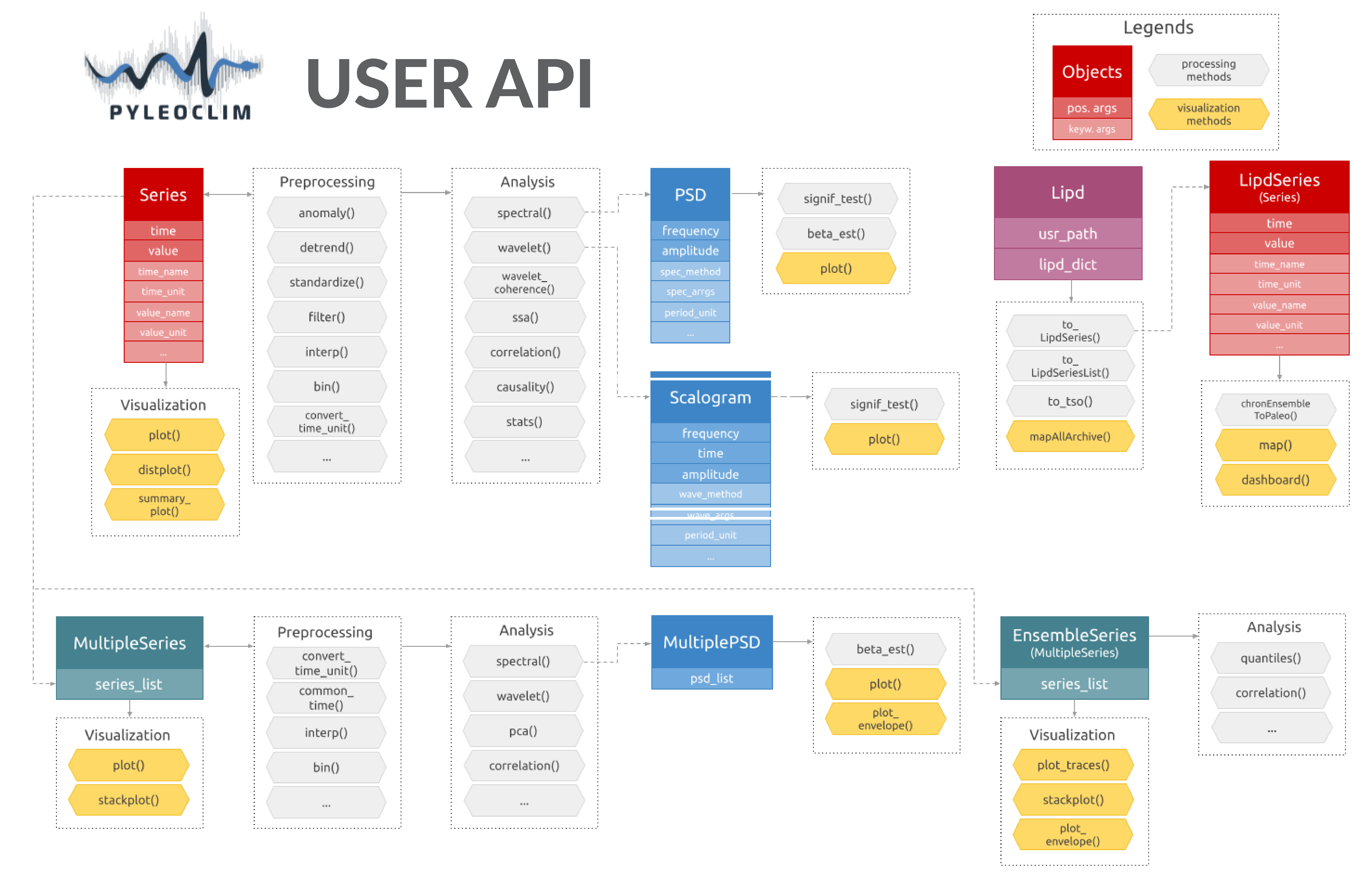
Pyleoclim User API

Pyleoclim, like a lot of other Python packages, follows an object-oriented design. It sounds fancy, but it really is quite simple. What this means for you is that we’ve gone through the trouble of coding up a lot of timeseries analysis methods that apply in various situations - so you don’t have to worry about that. These situations are described in classes, the beauty of which is called “inheritance” (see link above). Basically, it allows to define methods that will automatically apply to your dataset, as long as you put your data within one of those classes. A major advantage of object-oriented design is that you, the user, can harness the power of Pyleoclim methods in very few lines of code through the user API without ever having to get your hands dirty with our code (unless you want to, of course). The flipside is that any user would do well to understand Pyleoclim classes, what they are intended for, and what methods they support.

The following describes the various classes that undergird the Pyleoclim edifice.

Series (pyleoclim.Series)

class pyleoclim.core.series.Series(time, value, time_name=None, time_unit=None, value_name=None, value_unit=None, label=None, mean=None, clean_ts=True, log=None, verbose=False)[source]

The Series class describes the most basic objects in Pyleoclim. A Series is a simple dictionary that contains 3 things:

a series of real-valued numbers;
a time axis at which those values were measured/simulated ;
optionally, some metadata about both axes, like units, labels and the like.

How to create and manipulate such objects is described in a short example below, while this notebook demonstrates how to apply various Pyleoclim methods to Series objects.

Parameters:

time (list or numpy.array) – independent variable (t)
value (list of numpy.array) – values of the dependent variable (y)
time_unit (string) – Units for the time vector (e.g., ‘years’). Default is ‘years’
time_name (string) – Name of the time vector (e.g., ‘Time’,’Age’). Default is None. This is used to label the time axis on plots
value_name (string) – Name of the value vector (e.g., ‘temperature’) Default is None
value_unit (string) – Units for the value vector (e.g., ‘deg C’) Default is None
label (string) – Name of the time series (e.g., ‘Nino 3.4’) Default is None
clean_ts (boolean flag) – set to True to remove the NaNs and make time axis strictly prograde with duplicated timestamps reduced by averaging the values Default is True
log (dict) –
True (If keep_log is set to) –
kept. (then a log of the transformations made to the timeseries will be) –
verbose (bool) – If True, will print warning messages if there is any

Examples

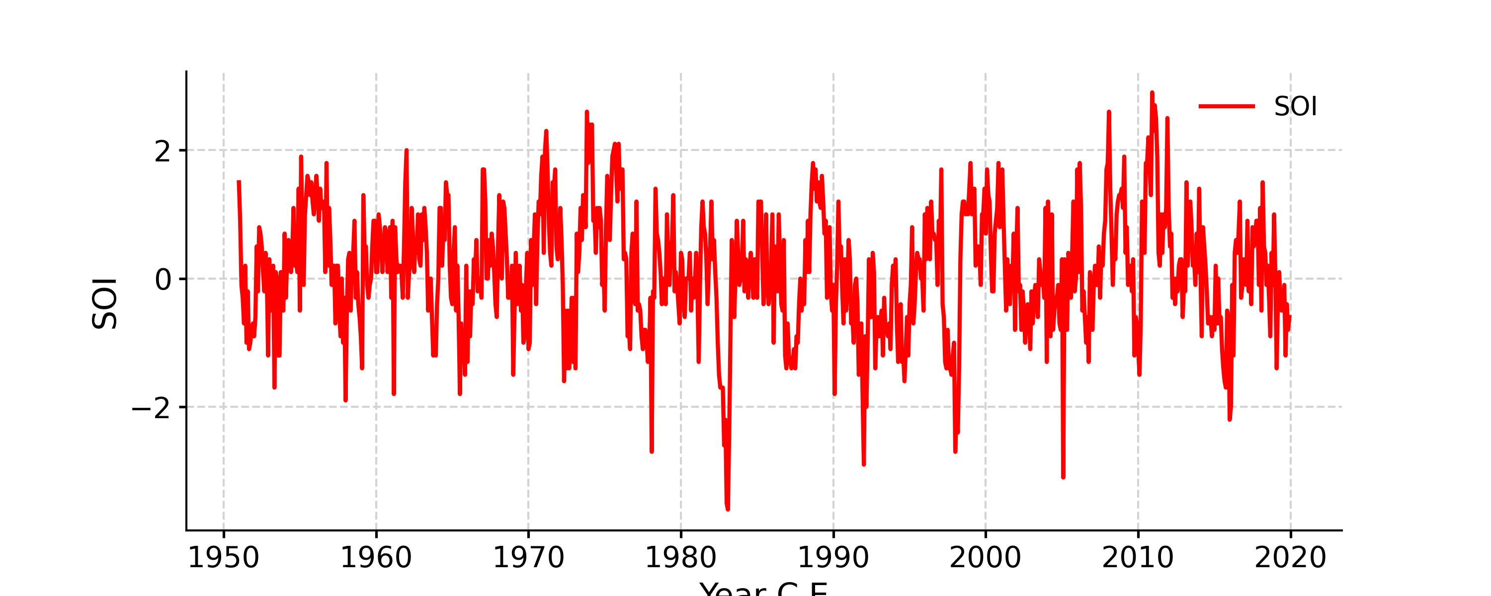
In this example, we import the Southern Oscillation Index (SOI) into a pandas dataframe and create a Series object.

In [1]: import pyleoclim as pyleo

In [2]: import pandas as pd

In [3]: data=pd.read_csv(
   ...:     'https://raw.githubusercontent.com/LinkedEarth/Pyleoclim_util/Development/example_data/soi_data.csv',
   ...:     skiprows=0, header=1
   ...: )
   ...: 

In [4]: time=data.iloc[:,1]

In [5]: value=data.iloc[:,2]

In [6]: ts=pyleo.Series(
   ...:     time=time, value=value,
   ...:     time_name='Year (CE)', value_name='SOI', label='Southern Oscillation Index'
   ...: )
   ...: 

In [7]: ts
Out[7]: <pyleoclim.core.series.Series at 0x7f17f5979870>

In [8]: ts.__dict__.keys()
Out[8]: dict_keys(['log', 'time', 'value', 'time_name', 'time_unit', 'value_name', 'value_unit', 'label', 'mean'])

For a quick look at the values, one may use the print() method. We do so below for a short slice of the data so as not to overwhelm the display:

In [9]: print(ts.slice([1982,1983]))
  Year (CE)    SOI
-----------  -----
     1.2
08    0.3
17    0.6
25    0.1
33   -0.3
42   -1
5    -1.5
58   -1.7
67   -1.7
75   -1.7
83   -2.6
92   -2.2
    -3.5
Length: 13

Methods

`bin`([keep_log])	Bin values in a time series
`causality`(target_series[, method, timespan, ...])	Perform causality analysis with the target timeseries. Specifically, whether there is information in the target series that influenced the original series.
`center`([timespan, keep_log])	Centers the series (i.e.
`clean`([verbose, keep_log])	Clean up the timeseries by removing NaNs and sort with increasing time points
`convert_time_unit`([time_unit, keep_log])	Convert the time unit of the Series object
`copy`()	Make a copy of the Series object
`correlation`(target_series[, timespan, ...])	Estimates the Pearson's correlation and associated significance between two non IID time series
`detrend`([method, keep_log])	Detrend Series object
`fill_na`([timespan, dt, keep_log])	Fill NaNs into the timespan
`filter`([cutoff_freq, cutoff_scale, method, ...])	Filtering methods for Series objects using four possible methods:
`flip`([axis, keep_log])	Flips the Series along one or both axes
`gaussianize`([keep_log])	Gaussianizes the timeseries (i.e.
`gkernel`([step_type, keep_log])	Coarse-grain a Series object via a Gaussian kernel.
`histplot`([figsize, title, savefig_settings, ...])	Plot the distribution of the timeseries values
`interp`([method, keep_log])	Interpolate a Series object onto a new time axis
`is_evenly_spaced`([tol])	Check if the Series time axis is evenly-spaced, within tolerance
`make_labels`()	Initialization of plot labels based on Series metadata
`outliers`([method, remove, settings, ...])	Remove outliers from timeseries data
`plot`([figsize, marker, markersize, color, ...])	Plot the timeseries
`segment`([factor])	Gap detection
`slice`(timespan)	Slicing the timeseries with a timespan (tuple or list)
`sort`([verbose, keep_log])	Ensure timeseries is aligned to a prograde axis.
`spectral`([method, freq_method, freq_kwargs, ...])	Perform spectral analysis on the timeseries
`ssa`([M, nMC, f, trunc, var_thresh])	Singular Spectrum Analysis
`standardize`([keep_log, scale])	Standardizes the series ((i.e.
`stats`()	Compute basic statistics from a Series
`stripes`(ref_period[, LIM, thickness, ...])	Represents the Series as an Ed Hawkins "stripes" pattern
`summary_plot`(psd, scalogram[, figsize, ...])	Produce summary plot of timeseries.
`surrogates`([method, number, length, seed, ...])	Generate surrogates with increasing time axis
`wavelet`([method, settings, freq_method, ...])	Perform wavelet analysis on a timeseries
`wavelet_coherence`(target_series[, method, ...])	Performs wavelet coherence analysis with the target timeseries

bin(keep_log=False, **kwargs)[source]

Bin values in a time series

Parameters:

keep_log (Boolean) – if True, adds this step and its parameters to the series log.
kwargs – Arguments for binning function. See pyleoclim.utils.tsutils.bin for details

Returns:

new – An binned Series object

Return type:

Series

See also

pyleoclim.utils.tsutils.bin: bin the series values into evenly-spaced time bins

causality(target_series, method='liang', timespan=None, settings=None, common_time_kwargs=None)[source]

Perform causality analysis with the target timeseries. Specifically, whether there is information in the target series that influenced the original series.: If the two series have different time axes, they are first placed on a common timescale (in ascending order).

Parameters:

target_series (Series) – A pyleoclim Series object on which to compute causality
method ({'liang', 'granger'}) – The causality method to use.
timespan (tuple) – The time interval over which to perform the calculation
settings (dict) – Parameters associated with the causality methods. Note that each method has different parameters. See individual methods for details
common_time_kwargs (dict) – Parameters for the method MultipleSeries.common_time(). Will use interpolation by default.

Returns:

res – Dictionary containing the results of the the causality analysis. See indivudal methods for details

Return type:

dict

See also

pyleoclim.utils.causality.liang_causality: Liang causality
pyleoclim.utils.causality.granger_causality: Granger causality

Examples

Liang causality

In [1]: import pyleoclim as pyleo

In [2]: import pandas as pd

In [3]: data=pd.read_csv('https://raw.githubusercontent.com/LinkedEarth/Pyleoclim_util/Development/example_data/wtc_test_data_nino.csv')

In [4]: t=data.iloc[:,0]

In [5]: air=data.iloc[:,1]

In [6]: nino=data.iloc[:,2]

In [7]: ts_nino=pyleo.Series(time=t,value=nino)

In [8]: ts_air=pyleo.Series(time=t,value=air)

In [9]: fig, ax = ts_nino.plot(title='NINO3 -- SST Anomalies')

In [10]: pyleo.closefig(fig)

In [11]: fig, ax = ts_air.plot(title='Deasonalized All Indian Rainfall Index')

In [12]: pyleo.closefig(fig)

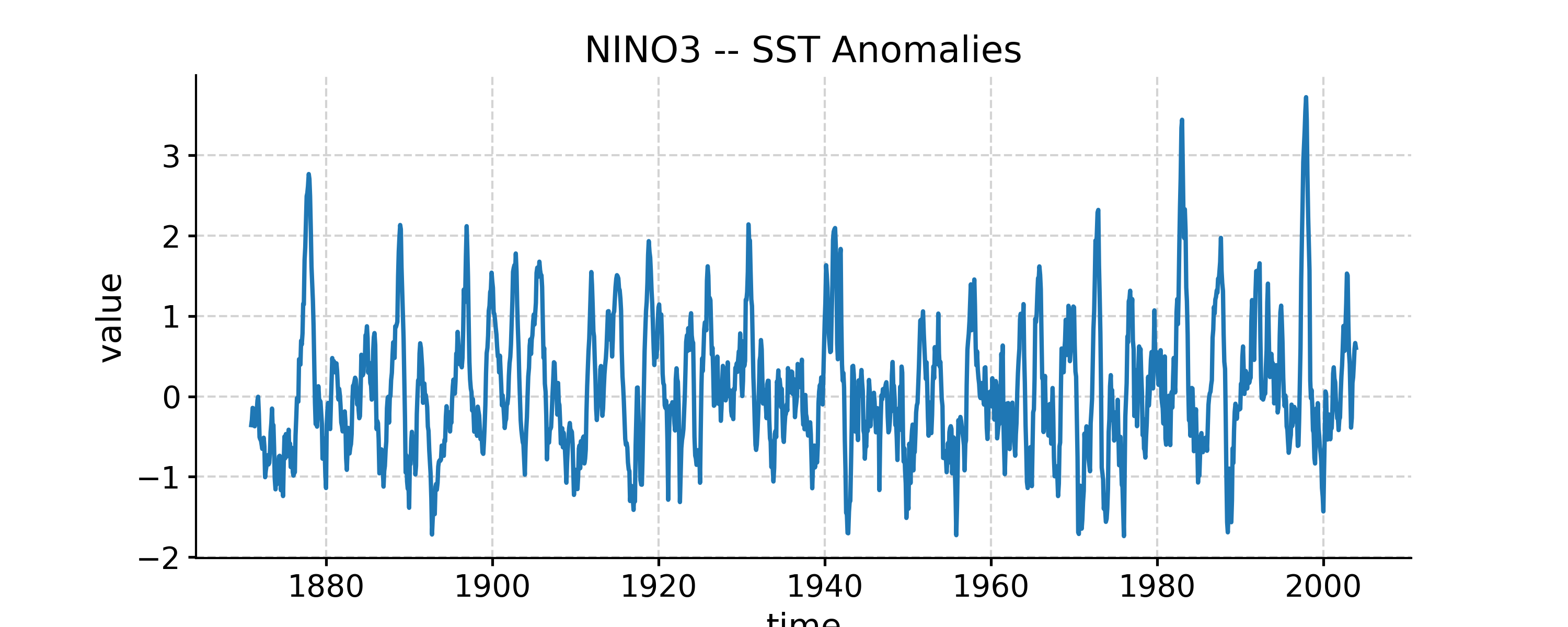
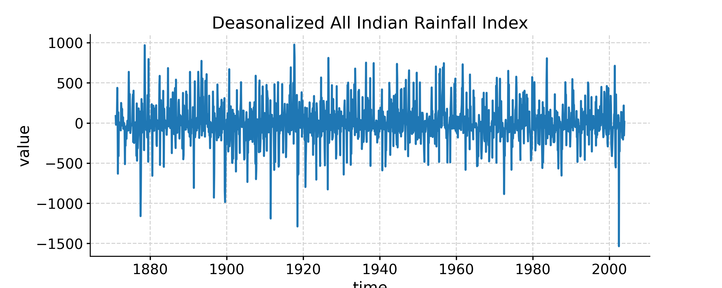
We use the specific params below to lighten computations; you may drop settings for real work

In [13]: liang_N2A = ts_air.causality(ts_nino, settings={'nsim': 20, 'signif_test': 'isopersist'})

In [14]: print(liang_N2A)
{'T21': 0.0164454802863363, 'tau21': 0.011968992003857074, 'Z': 1.3740071244960856, 'dH1_star': -0.6359251528278842, 'dH1_noise': 0.35210585516825876, 'signif_qs': [0.005, 0.025, 0.05, 0.95, 0.975, 0.995], 'T21_noise': array([-1.81031631e-05, -1.81031631e-05, -9.41450238e-06,  3.21912487e-03,
        4.64929404e-03,  4.64929404e-03]), 'tau21_noise': array([-1.37510439e-05, -1.37510439e-05, -7.17184550e-06,  2.35987959e-03,
        3.39638817e-03,  3.39638817e-03])}

In [15]: liang_A2N = ts_nino.causality(ts_air, settings={'nsim': 20, 'signif_test': 'isopersist'})

In [16]: print(liang_A2N)
{'T21': 0.0058402187949833225, 'tau21': 0.04731826159975569, 'Z': 0.12342420447275004, 'dH1_star': -0.5094709112673714, 'dH1_noise': 0.4432108271328728, 'signif_qs': [0.005, 0.025, 0.05, 0.95, 0.975, 0.995], 'T21_noise': array([-0.00048221, -0.00048221, -0.0004216 ,  0.00025923,  0.00028671,
        0.00028671]), 'tau21_noise': array([-0.00301088, -0.00301088, -0.00299985,  0.00226293,  0.00243632,
        0.00243632])}

In [17]: liang_N2A['T21']/liang_A2N['T21']
Out[17]: 2.815901400896619

Both information flows (T21) are positive, but the flow from NINO3 to AIR is about 3x as large as the other way around, suggesting that NINO3 influences AIR much more than the other way around, which conforms to physical intuition.

To implement Granger causality, simply specfiy the method:

In [18]: granger_A2N = ts_nino.causality(ts_air, method='granger')

Granger Causality
number of lags (no zero) 1
ssr based F test:         F=20.8492 , p=0.0000  , df_denom=1592, df_num=1
ssr based chi2 test:   chi2=20.8885 , p=0.0000  , df=1
likelihood ratio test: chi2=20.7529 , p=0.0000  , df=1
parameter F test:         F=20.8492 , p=0.0000  , df_denom=1592, df_num=1

In [19]: granger_N2A = ts_air.causality(ts_nino, method='granger')

Granger Causality
number of lags (no zero) 1
ssr based F test:         F=18.6927 , p=0.0000  , df_denom=1592, df_num=1
ssr based chi2 test:   chi2=18.7280 , p=0.0000  , df=1
likelihood ratio test: chi2=18.6189 , p=0.0000  , df=1
parameter F test:         F=18.6927 , p=0.0000  , df_denom=1592, df_num=1

Note that the output is fundamentally different for the two methods. Granger causality cannot discriminate between NINO3 -> AIR or AIR -> NINO3, in this case. This is not unusual, and one reason why it is no longer in wide use.

center(timespan=None, keep_log=False)[source]

Centers the series (i.e. renove its estimated mean)

Parameters:

timespan (tuple or list) – The timespan over which the mean must be estimated. In the form [a, b], where a, b are two points along the series’ time axis.
keep_log (Boolean) – if True, adds the previous mean and method parameters to the series log.

Returns:

new – The centered series object

Return type:

Series

clean(verbose=False, keep_log=False)[source]

Clean up the timeseries by removing NaNs and sort with increasing time points

Parameters:

verbose (bool) – If True, will print warning messages if there is any
keep_log (Boolean) – if True, adds this step and its parameters to the series log.

Returns:

new – Series object with removed NaNs and sorting

Return type:

Series

convert_time_unit(time_unit='years', keep_log=False)[source]

Convert the time unit of the Series object

Parameters:

time_unit (str) –
the target time unit, possible input: {

’year’, ‘years’, ‘yr’, ‘yrs’, ‘y BP’, ‘yr BP’, ‘yrs BP’, ‘year BP’, ‘years BP’, ‘ky BP’, ‘kyr BP’, ‘kyrs BP’, ‘ka BP’, ‘ka’, ‘my BP’, ‘myr BP’, ‘myrs BP’, ‘ma BP’, ‘ma’,

}
keep_log (Boolean) – if True, adds this step and its parameter to the series log.

Examples

In [1]: import pyleoclim as pyleo

In [2]: import pandas as pd

In [3]: data = pd.read_csv(
   ...:     'https://raw.githubusercontent.com/LinkedEarth/Pyleoclim_util/Development/example_data/soi_data.csv',
   ...:     skiprows=0, header=1)
   ...: 

In [4]: time = data.iloc[:,1]

In [5]: value = data.iloc[:,2]

In [6]: ts = pyleo.Series(time=time, value=value, time_unit='years')

In [7]: new_ts = ts.convert_time_unit(time_unit='yrs BP')

In [8]: print('Original timeseries:')
Original timeseries:

In [9]: print('time unit:', ts.time_unit)
time unit: years

In [10]: print('time:', ts.time[:10])
time: [1951.       1951.083333 1951.166667 1951.25     1951.333333 1951.416667
 1951.5      1951.583333 1951.666667 1951.75    ]

In [11]: print()


In [12]: print('Converted timeseries:')
Converted timeseries:

In [13]: print('time unit:', new_ts.time_unit)
time unit: yrs BP

In [14]: print('time:', new_ts.time[:10])
time: [-69.916667 -69.833333 -69.75     -69.666667 -69.583333 -69.5
 -69.416667 -69.333333 -69.25     -69.166667]

copy()[source]

Make a copy of the Series object

Returns:: Series – A copy of the Series object
Return type:: Series

correlation(target_series, timespan=None, alpha=0.05, settings=None, common_time_kwargs=None, seed=None)[source]

Estimates the Pearson’s correlation and associated significance between two non IID time series

The significance of the correlation is assessed using one of the following methods:

‘ttest’: T-test adjusted for effective sample size.
‘isopersistent’: AR(1) modeling of x and y.
‘isospectral’: phase randomization of original inputs. (default)

The T-test is a parametric test, hence computationally cheap, but can only be performed in ideal circumstances. The others are non-parametric, but their computational requirements scale with the number of simulations.

The choise of significance test and associated number of Monte-Carlo simulations are passed through the settings parameter.

Parameters:

target_series (Series) – A pyleoclim Series object
timespan (tuple) – The time interval over which to perform the calculation
alpha (float) – The significance level (default: 0.05)
settings (dict) –
Parameters for the correlation function, including:

nsimint
the number of simulations (default: 1000)

methodstr, {‘ttest’,’isopersistent’,’isospectral’ (default)}
method for significance testing
common_time_kwargs (dict) – Parameters for the method MultipleSeries.common_time(). Will use interpolation by default.
seed (float or int) – random seed for isopersistent and isospectral methods

Returns:

corr – the result object, containing

rfloat
correlation coefficient
pfloat
the p-value
signifbool
true if significant; false otherwise Note that signif = True if and only if p <= alpha.
alphafloat
the significance level

Return type:

pyleoclim.Corr

See also

pyleoclim.utils.correlation.corr_sig: Correlation function
pyleoclim.multipleseries.common_time: Aligning time axes

Examples

Correlation between the Nino3.4 index and the Deasonalized All Indian Rainfall Index

In [1]: import pyleoclim as pyleo

In [2]: import pandas as pd

In [3]: data = pd.read_csv('https://raw.githubusercontent.com/LinkedEarth/Pyleoclim_util/Development/example_data/wtc_test_data_nino.csv')

In [4]: t = data.iloc[:, 0]

In [5]: air = data.iloc[:, 1]

In [6]: nino = data.iloc[:, 2]

In [7]: ts_nino = pyleo.Series(time=t, value=nino)

In [8]: ts_air = pyleo.Series(time=t, value=air)

# with `nsim=20` and default `method='isospectral'`
# set an arbitrary random seed to fix the result
In [9]: corr_res = ts_nino.correlation(ts_air, settings={'nsim': 20}, seed=2333)

In [10]: print(corr_res)
  correlation  p-value    signif. (α: 0.05)
-------------  ---------  -------------------
    -0.152394  < 1e-6     True


# using a simple t-test
# set an arbitrary random seed to fix the result
In [11]: corr_res = ts_nino.correlation(ts_air, settings={'method': 'ttest'})

In [12]: print(corr_res)
  correlation  p-value    signif. (α: 0.05)
-------------  ---------  -------------------
    -0.152394  < 1e-7     True


# using the method "isopersistent"
# set an arbitrary random seed to fix the result
In [13]: corr_res = ts_nino.correlation(ts_air, settings={'nsim': 20, 'method': 'isopersistent'}, seed=2333)

In [14]: print(corr_res)
  correlation  p-value    signif. (α: 0.05)
-------------  ---------  -------------------
    -0.152394  < 1e-4     True

detrend(method='emd', keep_log=False, **kwargs)[source]

Detrend Series object

Parameters:

method (str, optional) –
The method for detrending. The default is ‘emd’. Options include:
- ”linear”: the result of a n ordinary least-squares stright line fit to y is subtracted.
- ”constant”: only the mean of data is subtracted.
- ”savitzky-golay”, y is filtered using the Savitzky-Golay filters and the resulting filtered series is subtracted from y.
- ”emd” (default): Empirical mode decomposition. The last mode is assumed to be the trend and removed from the series
keep_log (Boolean) – if True, adds the removed trend and method parameters to the series log.
kwargs (dict) – Relevant arguments for each of the methods.

Returns:

new – Detrended Series object in “value”, with new field “trend” added

Return type:

Series

See also

pyleoclim.utils.tsutils.detrend: detrending wrapper functions

Examples

We will generate a harmonic signal with a nonlinear trend and use two detrending options to recover the original signal.

In [1]: import pyleoclim as pyleo

In [2]: import numpy as np

# Generate a mixed harmonic signal with known frequencies
In [3]: freqs=[1/20,1/80]

In [4]: time=np.arange(2001)

In [5]: signals=[]

In [6]: for freq in freqs:
   ...:     signals.append(np.cos(2*np.pi*freq*time))
   ...: 

In [7]: signal=sum(signals)

# Add a non-linear trend
In [8]: slope = 1e-5;  intercept = -1

In [9]: nonlinear_trend = slope*time**2 + intercept

# Add a modicum of white noise
In [10]: np.random.seed(2333)

In [11]: sig_var = np.var(signal)

In [12]: noise_var = sig_var / 2 #signal is twice the size of noise

In [13]: white_noise = np.random.normal(0, np.sqrt(noise_var), size=np.size(signal))

In [14]: signal_noise = signal + white_noise

# Place it all in a series object and plot it:
In [15]: ts = pyleo.Series(time=time,value=signal_noise + nonlinear_trend)

In [16]: fig, ax = ts.plot(title='Timeseries with nonlinear trend'); pyleo.closefig(fig)

# Detrending with default parameters (using EMD method with 1 mode)
In [17]: ts_emd1 = ts.detrend()

In [18]: ts_emd1.label = 'default detrending (EMD, last mode)'

In [19]: fig, ax = ts_emd1.plot(title='Detrended with EMD method'); ax.plot(time,signal_noise,label='target signal'); ax.legend(); pyleo.closefig(fig)

We see that the default function call results in a “hockey stick” at the end, which is undesirable. There is no automated way to fix this, but with a little trial and error, we find that removing the 2 smoothest modes performs reasonably well:

In [20]: ts_emd2 = ts.detrend(method='emd', n=2, keep_log=True)

In [21]: ts_emd2.label = 'EMD detrending, last 2 modes'

In [22]: fig, ax = ts_emd2.plot(title='Detrended with EMD (n=2)'); ax.plot(time,signal_noise,label='target signal'); ax.legend(); pyleo.closefig(fig)

Another option for removing a nonlinear trend is a Savitzky-Golay filter:

In [23]: ts_sg = ts.detrend(method='savitzky-golay')

In [24]: ts_sg.label = 'savitzky-golay detrending, default parameters'

In [25]: fig, ax = ts_sg.plot(title='Detrended with Savitzky-Golay filter'); ax.plot(time,signal_noise,label='target signal'); ax.legend(); pyleo.closefig(fig)

As we can see, the result is even worse than with EMD (default). Here it pays to look into the underlying method, which comes from SciPy. It turns out that by default, the Savitzky-Golay filter fits a polynomial to the last “window_length” values of the edges. By default, this value is close to the length of the series. Choosing a value 10x smaller fixes the problem here, though you will have to tinker with that parameter until you get the result you seek.

In [26]: ts_sg2 = ts.detrend(method='savitzky-golay',sg_kwargs={'window_length':201}, keep_log=True)

In [27]: ts_sg2.label = 'savitzky-golay detrending, window_length = 201'

In [28]: fig, ax = ts_sg2.plot(title='Detrended with Savitzky-Golay filter'); ax.plot(time,signal_noise,label='target signal'); ax.legend(); pyleo.closefig(fig)

Finally, the method returns the trend that was previous, so it can be added back in if need be.

In [29]: trend_ts = pyleo.Series(time = time, value = nonlinear_trend,
   ....:                         value_name= 'trend', label='original trend')
   ....: 

In [30]: fig, ax = trend_ts.plot(title='Trend recovery'); ax.plot(time,ts_emd2.log[1]['previous_trend'],label=ts_emd2.label); ax.plot(time,ts_sg2.log[1]['previous_trend'], label=ts_sg2.label); ax.legend(); pyleo.closefig(fig)

Both methods can recover the exponential trend, with some edge effects near the end that could be addressed by judicious padding.

fill_na(timespan=None, dt=1, keep_log=False)[source]

Fill NaNs into the timespan

Parameters:

timespan (tuple or list) – The list of time points for slicing, whose length must be 2. For example, if timespan = [a, b], then the sliced output includes one segment [a, b]. If None, will use the start point and end point of the original timeseries
dt (float) – The time spacing to fill the NaNs; default is 1.
keep_log (Boolean) – if True, adds this step and its parameters to the series log.

Returns:

new – The sliced Series object.

Return type:

Series

filter(cutoff_freq=None, cutoff_scale=None, method='butterworth', keep_log=False, **kwargs)[source]

Filtering methods for Series objects using four possible methods:

By default, this method implements a lowpass filter, though it can easily be turned into a bandpass or high-pass filter (see examples below).

Parameters:

method (str, {'savitzky-golay', 'butterworth', 'firwin', 'lanczos'}) – the filtering method - ‘butterworth’: a Butterworth filter (default = 3rd order) - ‘savitzky-golay’: Savitzky-Golay filter - ‘firwin’: finite impulse response filter design using the window method, with default window as Hamming - ‘lanczos’: Lanczos zero-phase filter
cutoff_freq (float or list) – The cutoff frequency only works with the Butterworth method. If a float, it is interpreted as a low-frequency cutoff (lowpass). If a list, it is interpreted as a frequency band (f1, f2), with f1 < f2 (bandpass). Note that only the Butterworth option (default) currently supports bandpass filtering.
cutoff_scale (float or list) – cutoff_freq = 1 / cutoff_scale The cutoff scale only works with the Butterworth method and when cutoff_freq is None. If a float, it is interpreted as a low-frequency (high-scale) cutoff (lowpass). If a list, it is interpreted as a frequency band (f1, f2), with f1 < f2 (bandpass).
keep_log (Boolean) – if True, adds this step and its parameters to the series log.
kwargs (dict) – a dictionary of the keyword arguments for the filtering method, see pyleoclim.utils.filter.savitzky_golay, pyleoclim.utils.filter.butterworth, pyleoclim.utils.filter.lanczos and pyleoclim.utils.filter.firwin for the details

Returns:

new

Return type:

Series

See also

pyleoclim.utils.filter.butterworth: Butterworth method
pyleoclim.utils.filter.savitzky_golay: Savitzky-Golay method
pyleoclim.utils.filter.firwin: FIR filter design using the window method
pyleoclim.utils.filter.lanczos: lowpass filter via Lanczos resampling

Examples

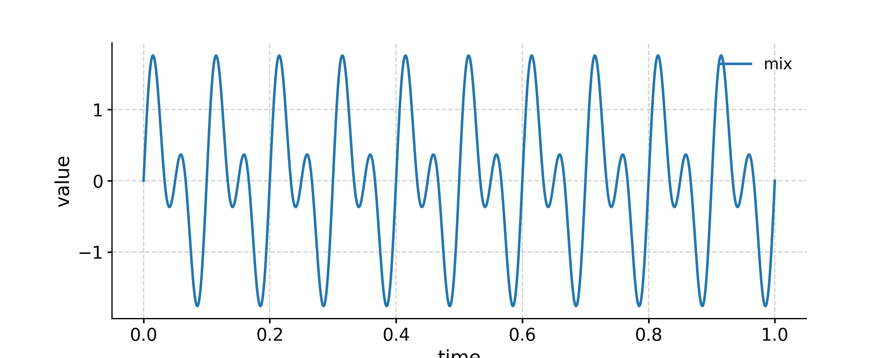
In the example below, we generate a signal as the sum of two signals with frequency 10 Hz and 20 Hz, respectively. Then we apply a low-pass filter with a cutoff frequency at 15 Hz, and compare the output to the signal of 10 Hz. After that, we apply a band-pass filter with the band 15-25 Hz, and compare the outcome to the signal of 20 Hz.

Generating the test data

In [1]: import pyleoclim as pyleo

In [2]: import numpy as np

In [3]: t = np.linspace(0, 1, 1000)

In [4]: sig1 = np.sin(2*np.pi*10*t)

In [5]: sig2 = np.sin(2*np.pi*20*t)

In [6]: sig = sig1 + sig2

In [7]: ts1 = pyleo.Series(time=t, value=sig1)

In [8]: ts2 = pyleo.Series(time=t, value=sig2)

In [9]: ts = pyleo.Series(time=t, value=sig)

In [10]: fig, ax = ts.plot(label='mix')

In [11]: ts1.plot(ax=ax, label='10 Hz')
Out[11]: <AxesSubplot: xlabel='time', ylabel='value'>

In [12]: ts2.plot(ax=ax, label='20 Hz')
Out[12]: <AxesSubplot: xlabel='time', ylabel='value'>

In [13]: ax.legend(loc='upper left', bbox_to_anchor=(0, 1.1), ncol=3)
Out[13]: <matplotlib.legend.Legend at 0x7f17ebf226b0>

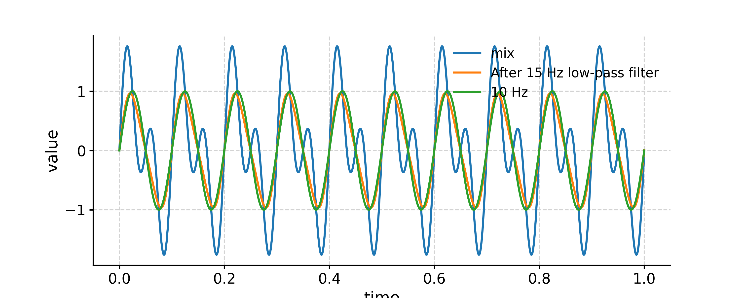
Applying a low-pass filter

In [14]: fig, ax = ts.plot(label='mix')

In [15]: ts.filter(cutoff_freq=15).plot(ax=ax, label='After 15 Hz low-pass filter')
Out[15]: <AxesSubplot: xlabel='time', ylabel='value'>

In [16]: ts1.plot(ax=ax, label='10 Hz')
Out[16]: <AxesSubplot: xlabel='time', ylabel='value'>

In [17]: ax.legend(loc='upper left', bbox_to_anchor=(0, 1.1), ncol=3)
Out[17]: <matplotlib.legend.Legend at 0x7f17ec1f3400>

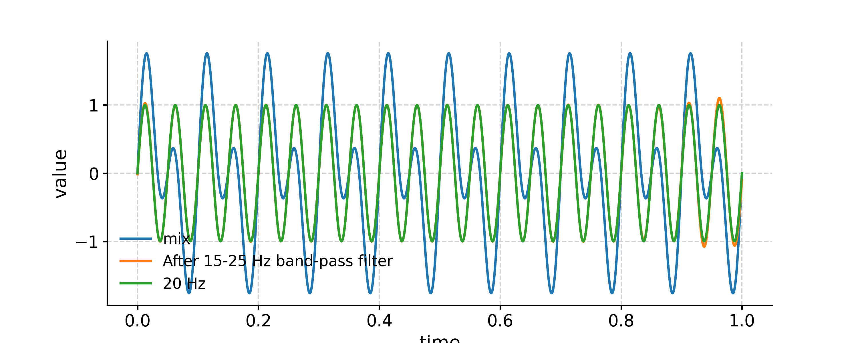
Applying a band-pass filter

In [18]: fig, ax = ts.plot(label='mix')

In [19]: ts.filter(cutoff_freq=[15, 25]).plot(ax=ax, label='After 15-25 Hz band-pass filter')
Out[19]: <AxesSubplot: xlabel='time', ylabel='value'>

In [20]: ts2.plot(ax=ax, label='20 Hz')
Out[20]: <AxesSubplot: xlabel='time', ylabel='value'>

In [21]: ax.legend(loc='upper left', bbox_to_anchor=(0, 1.1), ncol=3)
Out[21]: <matplotlib.legend.Legend at 0x7f17ec3d7d00>

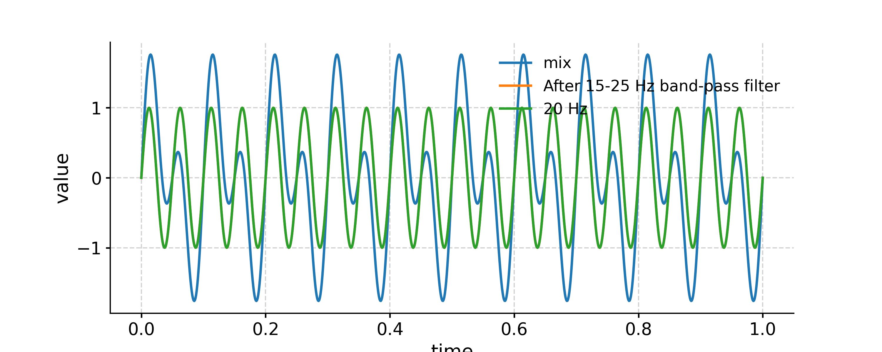
Above is using the default Butterworth filtering. To use FIR filtering with a window like Hanning is also simple:

In [22]: fig, ax = ts.plot(label='mix')

In [23]: ts.filter(cutoff_freq=[15, 25], method='firwin', window='hanning').plot(ax=ax, label='After 15-25 Hz band-pass filter')
Out[23]: <AxesSubplot: xlabel='time', ylabel='value'>

In [24]: ts2.plot(ax=ax, label='20 Hz')
Out[24]: <AxesSubplot: xlabel='time', ylabel='value'>

In [25]: ax.legend(loc='upper left', bbox_to_anchor=(0, 1.1), ncol=3)
Out[25]: <matplotlib.legend.Legend at 0x7f17f58a8d00>

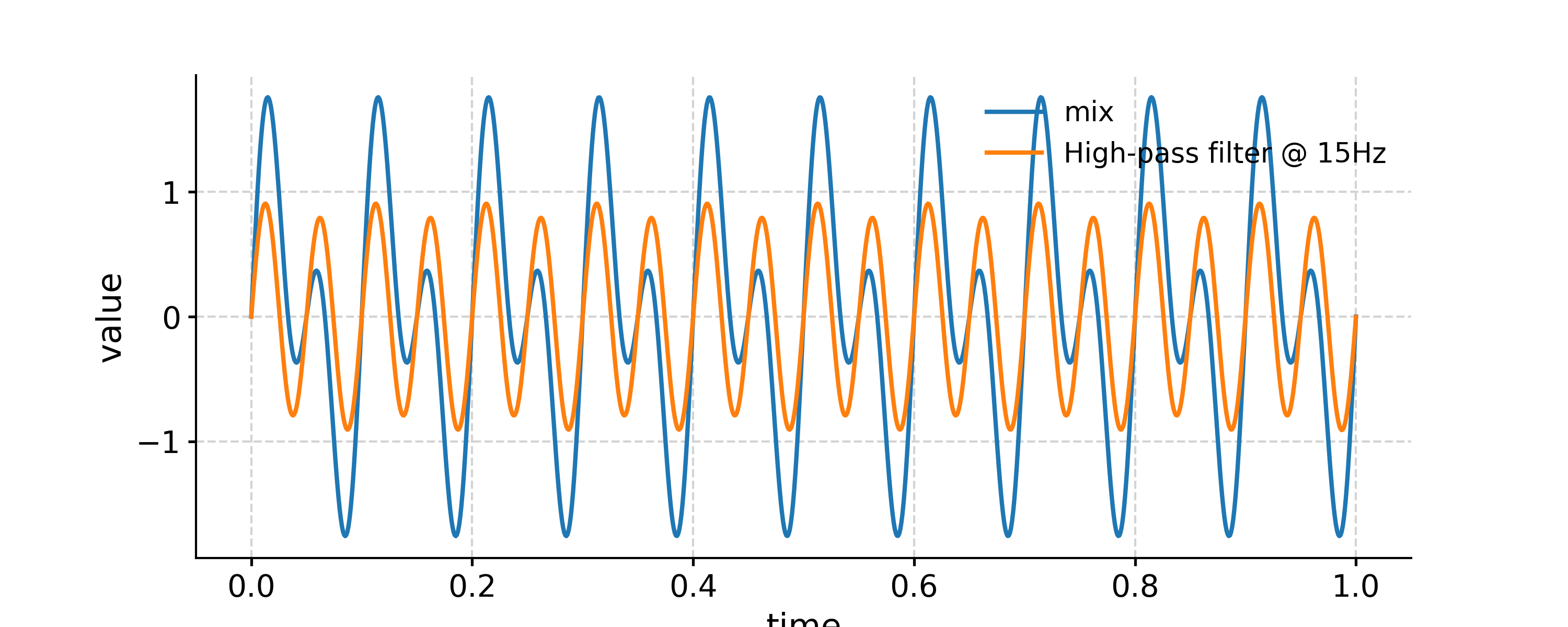
Applying a high-pass filter

In [26]: fig, ax = ts.plot(label='mix')

In [27]: ts_low  = ts.filter(cutoff_freq=15)

In [28]: ts_high = ts.copy()

In [29]: ts_high.value = ts.value - ts_low.value # subtract low-pass filtered series from original one

In [30]: ts_high.plot(label='High-pass filter @ 15Hz',ax=ax)
Out[30]: <AxesSubplot: xlabel='time', ylabel='value'>

In [31]: ax.legend(loc='upper left', bbox_to_anchor=(0, 1.1), ncol=3)
Out[31]: <matplotlib.legend.Legend at 0x7f17ec211d20>

flip(axis='value', keep_log=False)[source]

Flips the Series along one or both axes

Parameters:

axis (str, optional) – The axis along which the Series will be flipped. The default is ‘value’. Other acceptable options are ‘time’ or ‘both’. TODO: enable time flipping after paleopandas is released
keep_log (Boolean) – if True, adds this transformation to the series log.

Returns:

new – The flipped series object

Return type:

Series

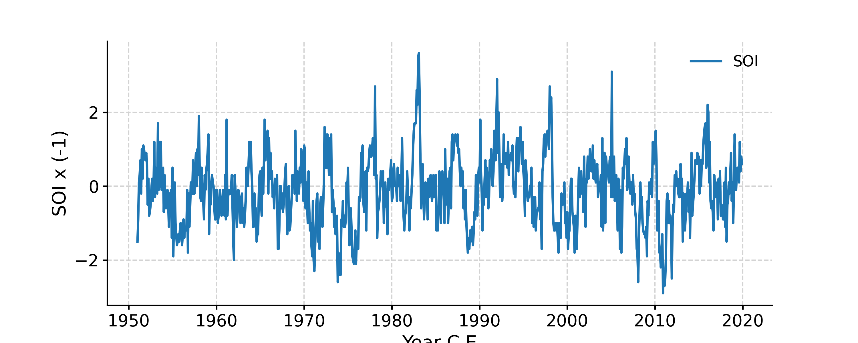
Examples

In [1]: import pyleoclim as pyleo

In [2]: import pandas as pd

In [3]: data = pd.read_csv('https://raw.githubusercontent.com/LinkedEarth/Pyleoclim_util/Development/example_data/soi_data.csv',skiprows=0,header=1)

In [4]: time = data.iloc[:,1]

In [5]: value = data.iloc[:,2]

In [6]: ts = pyleo.Series(time=time,value=value,time_name='Year C.E', value_name='SOI', label='SOI')

In [7]: tsf = ts.flip(keep_log=True)

In [8]: fig, ax = tsf.plot()

In [9]: tsf.log
Out[9]: 
({0: 'clean_ts', 'applied': True, 'verbose': False},
 {1: 'flip', 'applied': True, 'axis': 'value'})

In [10]: pyleo.closefig(fig)

gaussianize(keep_log=False)[source]

Gaussianizes the timeseries (i.e. maps its values to a standard normal)

Returns:

new (Series) – The Gaussianized series object
keep_log (Boolean) – if True, adds this transformation to the series log.

References

Emile-Geay, J., and M. Tingley (2016), Inferring climate variability from nonlinear proxies: application to palaeo-enso studies, Climate of the Past, 12 (1), 31–50, doi:10.5194/cp- 12-31-2016.

gkernel(step_type='median', keep_log=False, **kwargs)[source]

Coarse-grain a Series object via a Gaussian kernel.

Like .bin() this technique is conservative and uses the max space between points as the default spacing. Unlike .bin(), gkernel() uses a gaussian kernel to calculate the weighted average of the time series over these intervals.

Parameters:

step_type (str) – type of timestep: ‘mean’, ‘median’, or ‘max’ of the time increments
keep_log (Boolean) – if True, adds the step type and its keyword arguments to the series log.
kwargs – Arguments for kernel function. See pyleoclim.utils.tsutils.gkernel for details

Returns:

new – The coarse-grained Series object

Return type:

Series

See also

pyleoclim.utils.tsutils.gkernel: application of a Gaussian kernel

histplot(figsize=[10, 4], title=None, savefig_settings=None, ax=None, ylabel='KDE', vertical=False, edgecolor='w', **plot_kwargs)[source]

Plot the distribution of the timeseries values

Parameters:

figsize (list) – a list of two integers indicating the figure size
title (str) – the title for the figure
savefig_settings (dict) –
the dictionary of arguments for plt.savefig(); some notes below:
- ”path” must be specified; it can be any existed or non-existed path, with or without a suffix; if the suffix is not given in “path”, it will follow “format”
- ”format” can be one of {“pdf”, “eps”, “png”, “ps”}
ax (matplotlib.axis, optional) – A matplotlib axis
ylabel (str) – Label for the count axis
vertical ({True,False}) – Whether to flip the plot vertically
edgecolor (matplotlib.color) – The color of the edges of the bar
plot_kwargs (dict) – Plotting arguments for seaborn histplot: https://seaborn.pydata.org/generated/seaborn.histplot.html

See also

pyleoclim.utils.plotting.savefig: saving figure in Pyleoclim

Examples

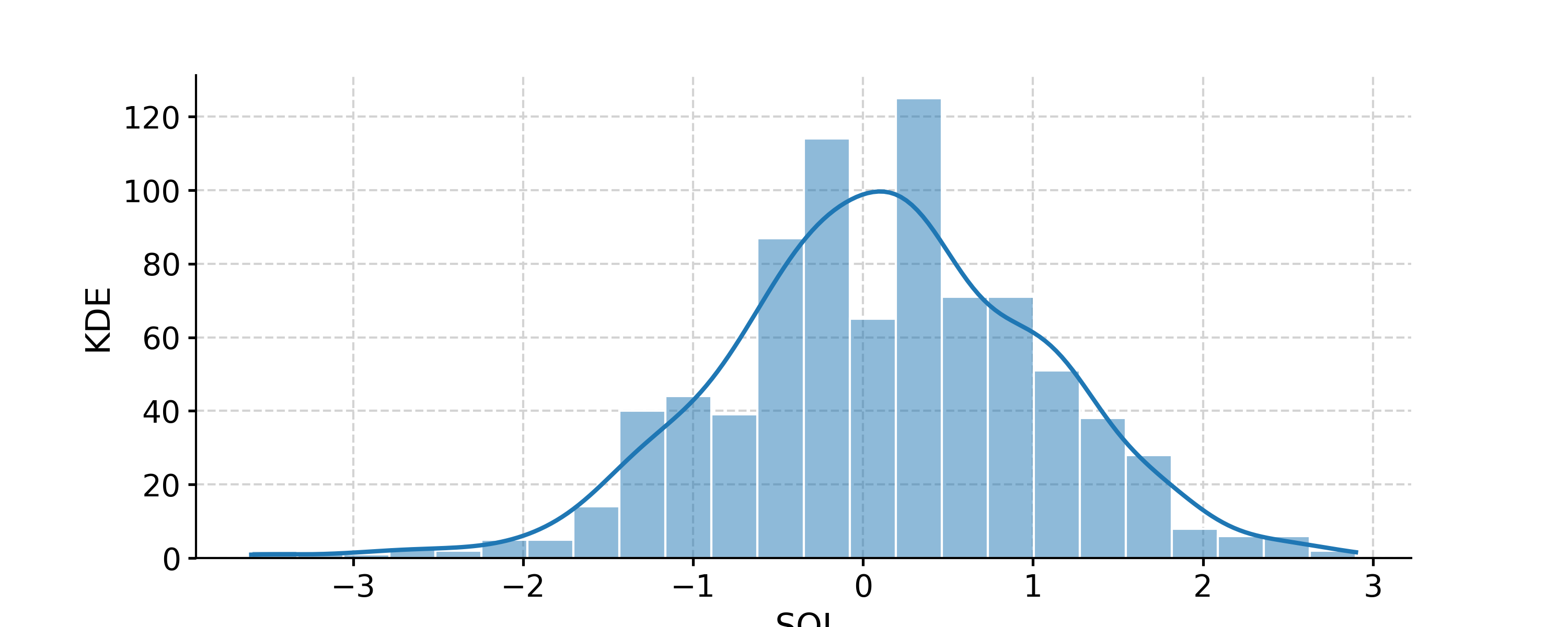
Distribution of the SOI record

In [1]: import pyleoclim as pyleo

In [2]: import pandas as pd

In [3]: data=pd.read_csv('https://raw.githubusercontent.com/LinkedEarth/Pyleoclim_util/Development/example_data/soi_data.csv',skiprows=0,header=1)

In [4]: time=data.iloc[:,1]

In [5]: value=data.iloc[:,2]

In [6]: ts=pyleo.Series(time=time,value=value,time_name='Year C.E', value_name='SOI', label='SOI')

In [7]: fig, ax = ts.plot()

In [8]: pyleo.closefig(fig)

In [9]: fig, ax = ts.histplot()

In [10]: pyleo.closefig(fig)

interp(method='linear', keep_log=False, **kwargs)[source]

Interpolate a Series object onto a new time axis

Parameters:

method ({‘linear’, ‘nearest’, ‘zero’, ‘slinear’, ‘quadratic’, ‘cubic’, ‘previous’, ‘next’}) – where ‘zero’, ‘slinear’, ‘quadratic’ and ‘cubic’ refer to a spline interpolation of zeroth, first, second or third order; ‘previous’ and ‘next’ simply return the previous or next value of the point) or as an integer specifying the order of the spline interpolator to use. Default is ‘linear’.
keep_log (Boolean) – if True, adds the method name and its parameters to the series log.
kwargs – Arguments specific to each interpolation function. See pyleoclim.utils.tsutils.interp for details

Returns:

new – An interpolated Series object

Return type:

Series

See also

pyleoclim.utils.tsutils.interp: interpolation function

is_evenly_spaced(tol=0.001)[source]

Check if the Series time axis is evenly-spaced, within tolerance

Parameters:: tol (float) – tolerance. If time increments are all within tolerance, the series is declared evenly-spaced. default = 1e-3
Returns:: res
Return type:: bool

make_labels()[source]

Initialization of plot labels based on Series metadata

Returns:

time_header (str) – Label for the time axis
value_header (str) – Label for the value axis

outliers(method='kmeans', remove=True, settings=None, fig_outliers=True, figsize_outliers=[10, 4], plotoutliers_kwargs=None, savefigoutliers_settings=None, fig_clusters=True, figsize_clusters=[10, 4], plotclusters_kwargs=None, savefigclusters_settings=None, keep_log=False)[source]

Remove outliers from timeseries data

Parameters:

method (str, {'kmeans','DBSCAN'}, optional) – The clustering method to use. The default is ‘kmeans’.
remove (bool, optional) – If True, removes the outliers. The default is True.
settings (dict, optional) – Specific arguments for the clustering functions. The default is None.
fig_outliers (bool, optional) – Whether to display the timeseries showing the outliers. The default is True.
figsize_outliers (list, optional) – The dimensions of the outliers figure. The default is [10,4].
plotoutliers_kwargs (dict, optional) – Arguments for the plot displaying the outliers. The default is None.
savefigoutliers_settings (dict, optional) –
Saving options for the outlier plot. The default is None. - “path” must be specified; it can be any existed or non-existed path,

with or without a suffix; if the suffix is not given in “path”, it will follow “format”
- ”format” can be one of {“pdf”, “eps”, “png”, “ps”}
fig_clusters (bool, optional) – Whether to display the clusters. The default is True.
figsize_clusters (list, optional) – The dimensions of the cluster figures. The default is [10,4].
plotclusters_kwargs (dict, optional) – Arguments for the cluster plot. The default is None.
savefigclusters_settings (dict, optional) –
Saving options for the cluster plot. The default is None. - “path” must be specified; it can be any existed or non-existed path,

with or without a suffix; if the suffix is not given in “path”, it will follow “format”
- ”format” can be one of {“pdf”, “eps”, “png”, “ps”}
keep_log (Boolean) – if True, adds the previous method parameters to the series log.

Returns:

ts – A new Series object witthout outliers if remove is True. Otherwise, returns the original timeseries

Return type:

Series

See also

pyleoclim.utils.tsutils.detect_outliers_DBSCAN: Outlier detection using the DBSCAN method
pyleoclim.utils.tsutils.detect_outliers_kmeans: Outlier detection using the kmeans method
pyleoclim.utils.tsutils.remove_outliers: Remove outliers from the series

plot(figsize=[10, 4], marker=None, markersize=None, color=None, linestyle=None, linewidth=None, xlim=None, ylim=None, label=None, xlabel=None, ylabel=None, title=None, zorder=None, legend=True, plot_kwargs=None, lgd_kwargs=None, alpha=None, savefig_settings=None, ax=None, invert_xaxis=False, invert_yaxis=False)[source]

Plot the timeseries

Parameters:

figsize (list) – a list of two integers indicating the figure size
marker (str) – e.g., ‘o’ for dots See [matplotlib.markers](https://matplotlib.org/stable/api/markers_api.html) for details
markersize (float) – the size of the marker
color (str, list) – the color for the line plot e.g., ‘r’ for red See [matplotlib colors](https://matplotlib.org/stable/gallery/color/color_demo.html) for details
linestyle (str) – e.g., ‘–’ for dashed line See [matplotlib.linestyles](https://matplotlib.org/stable/gallery/lines_bars_and_markers/linestyles.html) for details
linewidth (float) – the width of the line
label (str) – the label for the line
xlabel (str) – the label for the x-axis
ylabel (str) – the label for the y-axis
title (str) – the title for the figure
zorder (int) – The default drawing order for all lines on the plot
legend ({True, False}) – plot legend or not
invert_xaxis (bool, optional) – if True, the x-axis of the plot will be inverted
invert_yaxis (bool, optional) – same for the y-axis
plot_kwargs (dict) – the dictionary of keyword arguments for ax.plot() See [matplotlib.pyplot.plot](https://matplotlib.org/stable/api/_as_gen/matplotlib.pyplot.plot.html) for details
lgd_kwargs (dict) – the dictionary of keyword arguments for ax.legend() See [matplotlib.pyplot.legend](https://matplotlib.org/stable/api/_as_gen/matplotlib.pyplot.legend.html) for details
alpha (float) – Transparency setting
savefig_settings (dict) –
the dictionary of arguments for plt.savefig(); some notes below: - “path” must be specified; it can be any existed or non-existed path,

with or without a suffix; if the suffix is not given in “path”, it will follow “format”
- ”format” can be one of {“pdf”, “eps”, “png”, “ps”}
ax (matplotlib.axis, optional) – the axis object from matplotlib See [matplotlib.axes](https://matplotlib.org/api/axes_api.html) for details.

Returns:

fig (matplotlib.figure) – the figure object from matplotlib See [matplotlib.pyplot.figure](https://matplotlib.org/stable/api/figure_api.html) for details.
ax (matplotlib.axis) – the axis object from matplotlib See [matplotlib.axes](https://matplotlib.org/stable/api/axes_api.html) for details.

Notes

When ax is passed, the return will be ax only; otherwise, both fig and ax will be returned.

See also

pyleoclim.utils.plotting.savefig: saving a figure in Pyleoclim

Examples

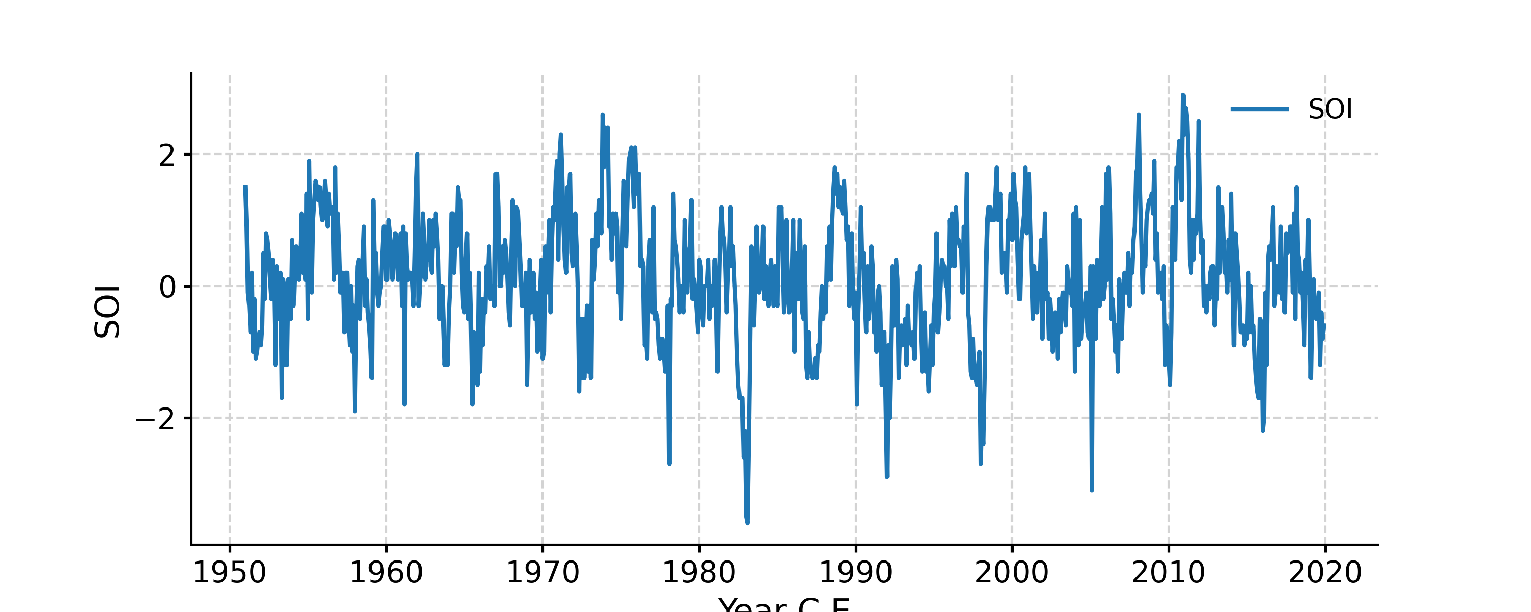
Plot the SOI record

In [1]: import pyleoclim as pyleo

In [2]: import pandas as pd

In [3]: data = pd.read_csv('https://raw.githubusercontent.com/LinkedEarth/Pyleoclim_util/Development/example_data/soi_data.csv',skiprows=0,header=1)

In [4]: time = data.iloc[:,1]

In [5]: value = data.iloc[:,2]

In [6]: ts = pyleo.Series(time=time,value=value,time_name='Year C.E', value_name='SOI', label='SOI')

In [7]: fig, ax = ts.plot()

In [8]: pyleo.closefig(fig)

Change the line color

In [9]: fig, ax = ts.plot(color='r')

In [10]: pyleo.closefig(fig)

Save the figure. Two options available, only one is needed:

Within the plotting command
After the figure has been generated

In [11]: fig, ax = ts.plot(color='k', savefig_settings={'path': 'ts_plot3.png'}); pyleo.closefig(fig)
Figure saved at: "ts_plot3.png"

In [12]: pyleo.savefig(fig,path='ts_plot3.png')
Figure saved at: "ts_plot3.png"

segment(factor=10)[source]

Gap detection

This function segments a timeseries into n number of parts following a gap: detection algorithm. The rule of gap detection is very simple: we define the intervals between time points as dts, then if dts[i] is larger than factor * dts[i-1], we think that the change of dts (or the gradient) is too large, and we regard it as a breaking point and divide the time series into two segments here

Parameters:: factor (float) – The factor that adjusts the threshold for gap detection
Returns:: res – If gaps were detected, returns the segments in a MultipleSeries object, else, returns the original timeseries.
Return type:: MultipleSeries or Series

slice(timespan)[source]

Slicing the timeseries with a timespan (tuple or list)

Parameters:: timespan (tuple or list) – The list of time points for slicing, whose length must be even. When there are n time points, the output Series includes n/2 segments. For example, if timespan = [a, b], then the sliced output includes one segment [a, b]; if timespan = [a, b, c, d], then the sliced output includes segment [a, b] and segment [c, d].
Returns:: new – The sliced Series object.
Return type:: Series

Examples

slice the SOI from 1972 to 1998

In [1]: import pyleoclim as pyleo

In [2]: import pandas as pd

In [3]: data = pd.read_csv('https://raw.githubusercontent.com/LinkedEarth/Pyleoclim_util/Development/example_data/soi_data.csv',skiprows=0,header=1)

In [4]: time = data.iloc[:,1]

In [5]: value = data.iloc[:,2]

In [6]: ts = pyleo.Series(time=time, value=value, time_name='Year C.E', value_name='SOI', label='SOI')

In [7]: ts_slice = ts.slice([1972, 1998])

In [8]: print("New time bounds:",ts_slice.time.min(),ts_slice.time.max())
New time bounds: 1972.0 1998.0

sort(verbose=False, keep_log=False)[source]

Ensure timeseries is aligned to a prograde axis.: If the time axis is prograde to begin with, no transformation is applied.

Parameters:

verbose (bool) – If True, will print warning messages if there is any
keep_log (Boolean) – if True, adds this step and its parameter to the series log.

Returns:

new – Series object with removed NaNs and sorting

Return type:

Series

spectral(method='lomb_scargle', freq_method='log', freq_kwargs=None, settings=None, label=None, scalogram=None, verbose=False)[source]

Perform spectral analysis on the timeseries

Parameters:

method (str;) – {‘wwz’, ‘mtm’, ‘lomb_scargle’, ‘welch’, ‘periodogram’, ‘cwt’}
freq_method (str) – {‘log’,’scale’, ‘nfft’, ‘lomb_scargle’, ‘welch’}
freq_kwargs (dict) – Arguments for frequency vector
settings (dict) – Arguments for the specific spectral method
label (str) – Label for the PSD object
scalogram (pyleoclim.core.series.Series.Scalogram) – The return of the wavelet analysis; effective only when the method is ‘wwz’ or ‘cwt’
verbose (bool) – If True, will print warning messages if there is any

Returns:

psd – A PSD object

Return type:

PSD

See also

pyleoclim.utils.spectral.mtm: Spectral analysis using the Multitaper approach
pyleoclim.utils.spectral.lomb_scargle: Spectral analysis using the Lomb-Scargle method
pyleoclim.utils.spectral.welch: Spectral analysis using the Welch segement approach
pyleoclim.utils.spectral.periodogram: Spectral anaysis using the basic Fourier transform
pyleoclim.utils.spectral.wwz_psd: Spectral analysis using the Wavelet Weighted Z transform
pyleoclim.utils.spectral.cwt_psd: Spectral analysis using the continuous Wavelet Transform as implemented by Torrence and Compo
pyleoclim.utils.spectral.make_freq_vector: Functions to create the frequency vector
pyleoclim.utils.tsutils.detrend: Detrending function
pyleoclim.core.psds.PSD: PSD object
pyleoclim.core.psds.MultiplePSD: Multiple PSD object

Examples

Calculate the spectrum of SOI using the various methods and compute significance

In [1]: import pyleoclim as pyleo

In [2]: import pandas as pd

In [3]: data = pd.read_csv('https://raw.githubusercontent.com/LinkedEarth/Pyleoclim_util/Development/example_data/soi_data.csv',skiprows=0,header=1)

In [4]: time = data.iloc[:,1]

In [5]: value = data.iloc[:,2]

In [6]: ts = pyleo.Series(time=time, value=value, time_name='Year C.E', value_name='SOI', label='SOI')

# Standardize the time series
In [7]: ts_std = ts.standardize()

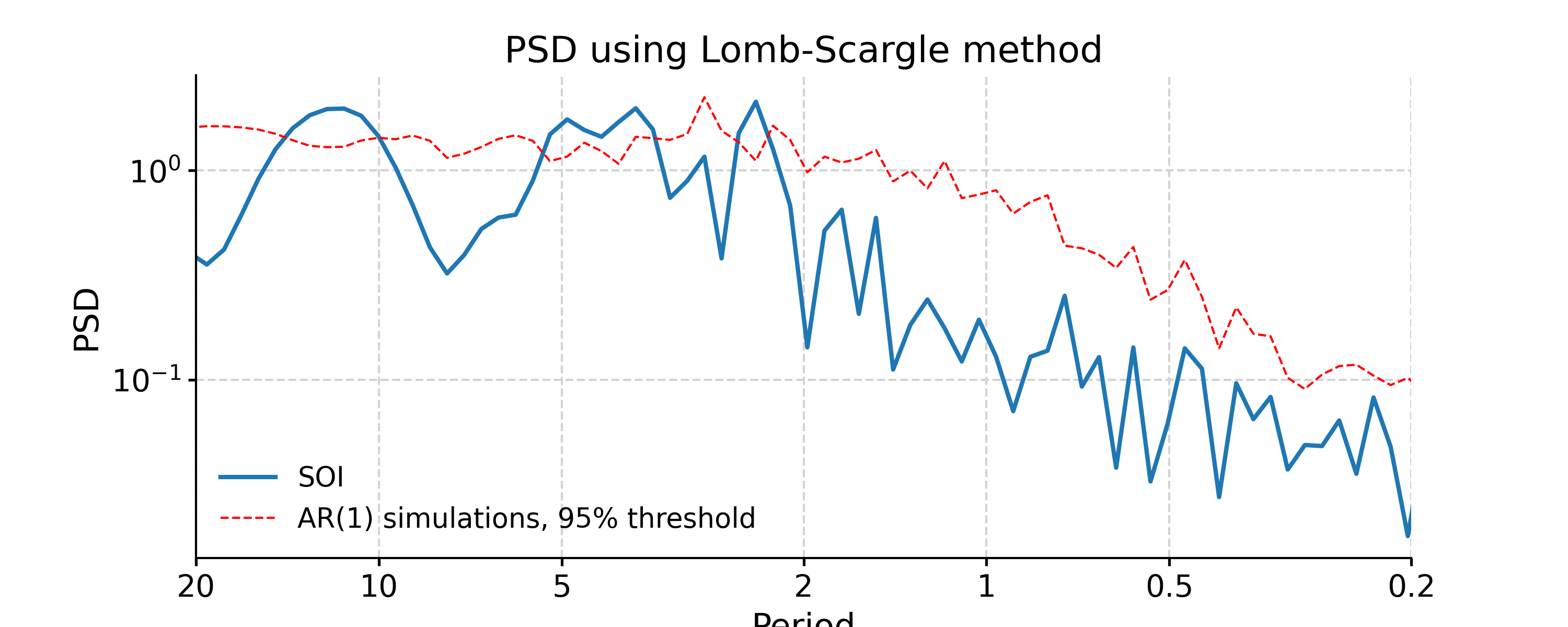
Lomb-Scargle

In [8]: psd_ls = ts_std.spectral(method='lomb_scargle')

In [9]: psd_ls_signif = psd_ls.signif_test(number=20) #in practice, need more AR1 simulations

In [10]: fig, ax = psd_ls_signif.plot(title='PSD using Lomb-Scargle method')

In [11]: pyleo.closefig(fig)

We may pass in method-specific arguments via “settings”, which is a dictionary. For instance, to adjust the number of overlapping segment for Lomb-Scargle, we may specify the method-specific argument “n50”; to adjust the frequency vector, we may modify the “freq_method” or modify the method-specific argument “freq”.

In [12]: import numpy as np

In [13]: psd_LS_n50 = ts_std.spectral(method='lomb_scargle', settings={'n50': 4})  # c=1e-2 yields lower frequency resolution

In [14]: psd_LS_freq = ts_std.spectral(method='lomb_scargle', settings={'freq': np.linspace(1/20, 1/0.2, 51)})

In [15]: psd_LS_LS = ts_std.spectral(method='lomb_scargle', freq_method='lomb_scargle')  # with frequency vector generated using REDFIT method

In [16]: fig, ax = psd_LS_n50.plot(
   ....:     title='PSD using Lomb-Scargle method with 4 overlapping segments',
   ....:     label='settings={"n50": 4}')
   ....: 

In [17]: psd_ls.plot(ax=ax, label='settings={"n50": 3}', marker='o')
Out[17]: <AxesSubplot: title={'center': 'PSD using Lomb-Scargle method with 4 overlapping segments'}, xlabel='Period', ylabel='PSD'>

In [18]: fig, ax = psd_LS_freq.plot(
   ....:     title='PSD using Lomb-Scargle method with different frequency vectors',
   ....:     label='freq=np.linspace(1/20, 1/0.2, 51)', marker='o')
   ....: 

In [19]: psd_ls.plot(ax=ax, label='freq_method="log"', marker='o')
Out[19]: <AxesSubplot: title={'center': 'PSD using Lomb-Scargle method with different frequency vectors'}, xlabel='Period', ylabel='PSD'>

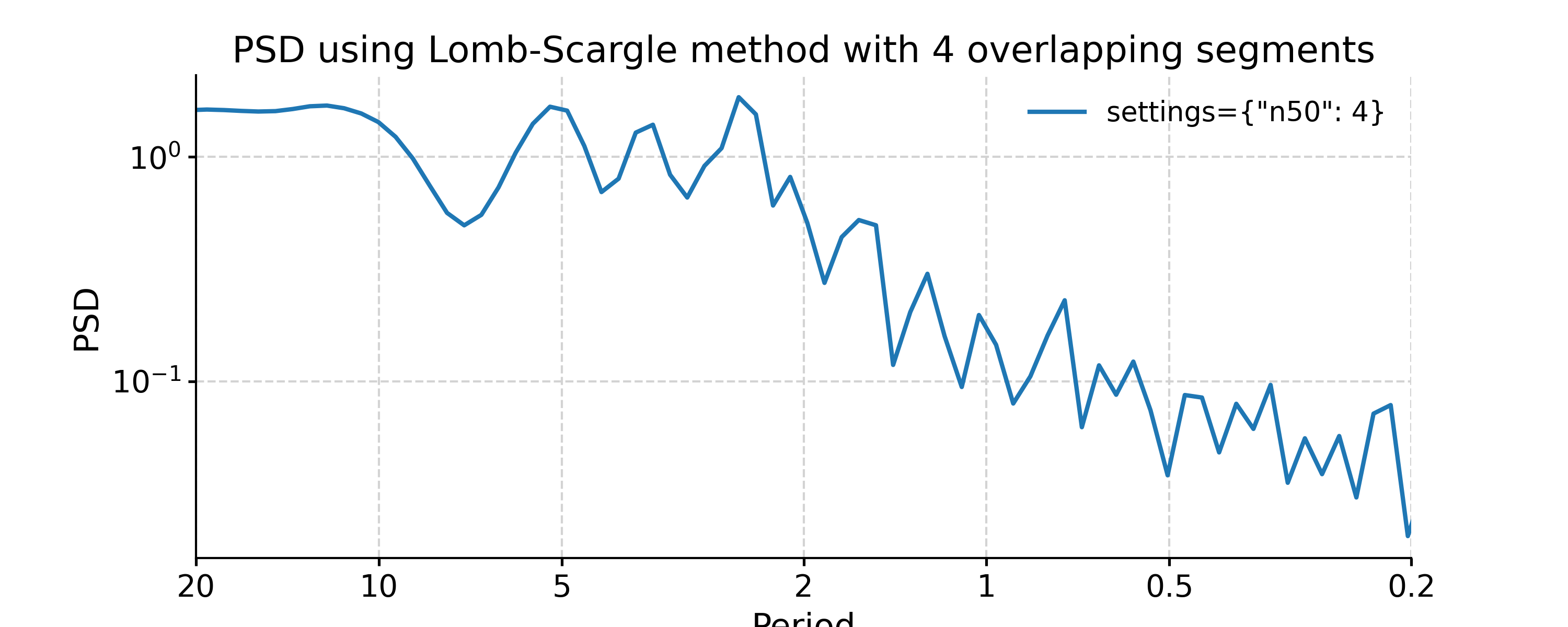
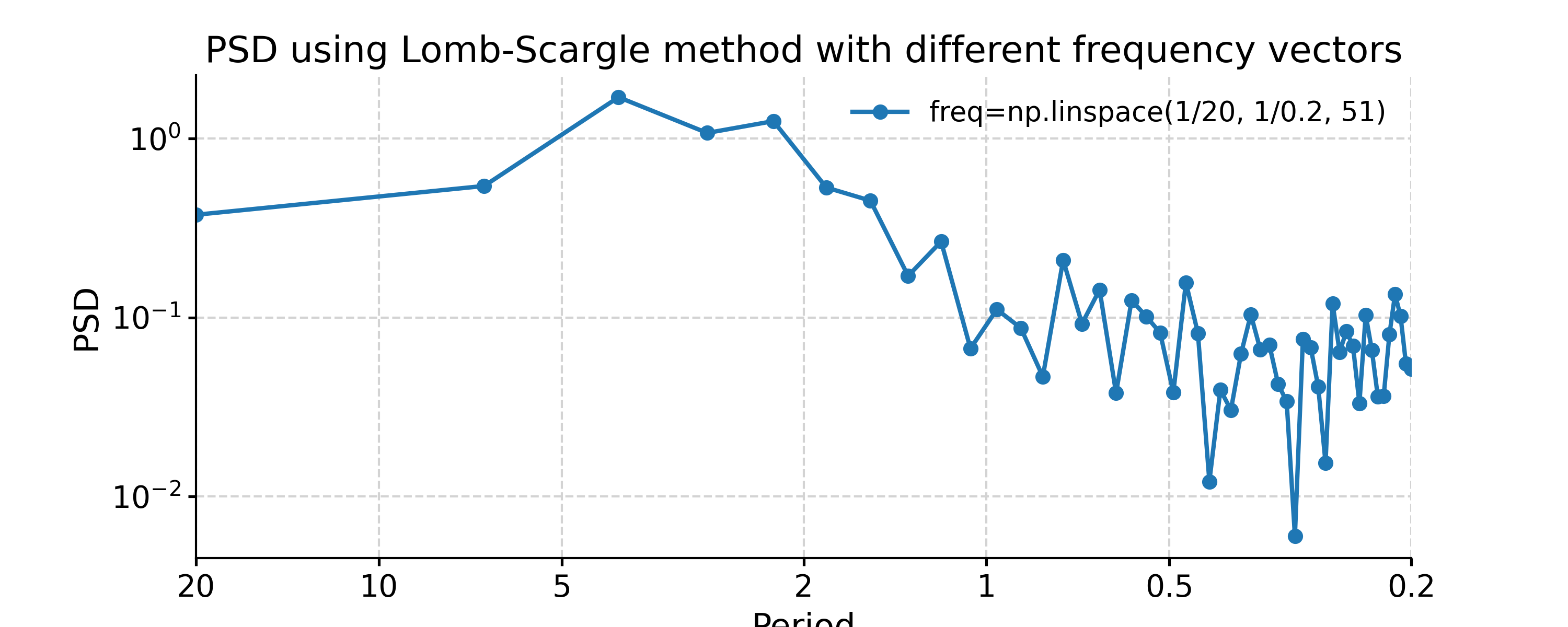
You may notice the differences in the PSD curves regarding smoothness and the locations of the analyzed period points.

For other method-specific arguments, please look up the specific methods in the “See also” section.

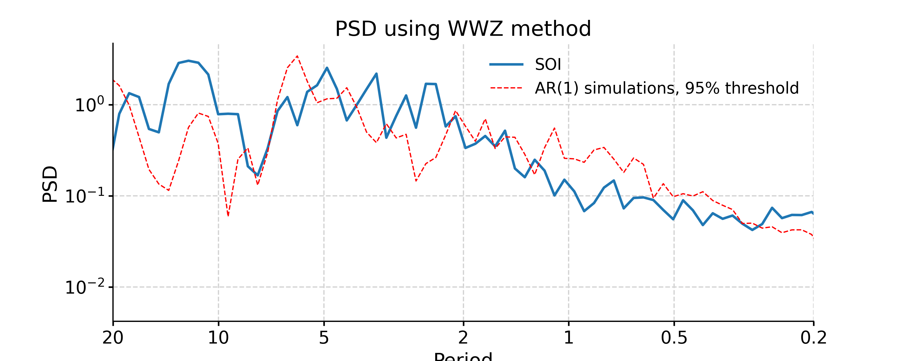
WWZ

In [20]: psd_wwz = ts_std.spectral(method='wwz')  # wwz is the default method

In [21]: psd_wwz_signif = psd_wwz.signif_test(number=1)  # significance test; for real work, should use number=200 or even larger

In [22]: fig, ax = psd_wwz_signif.plot(title='PSD using WWZ method')

In [23]: pyleo.closefig(fig)

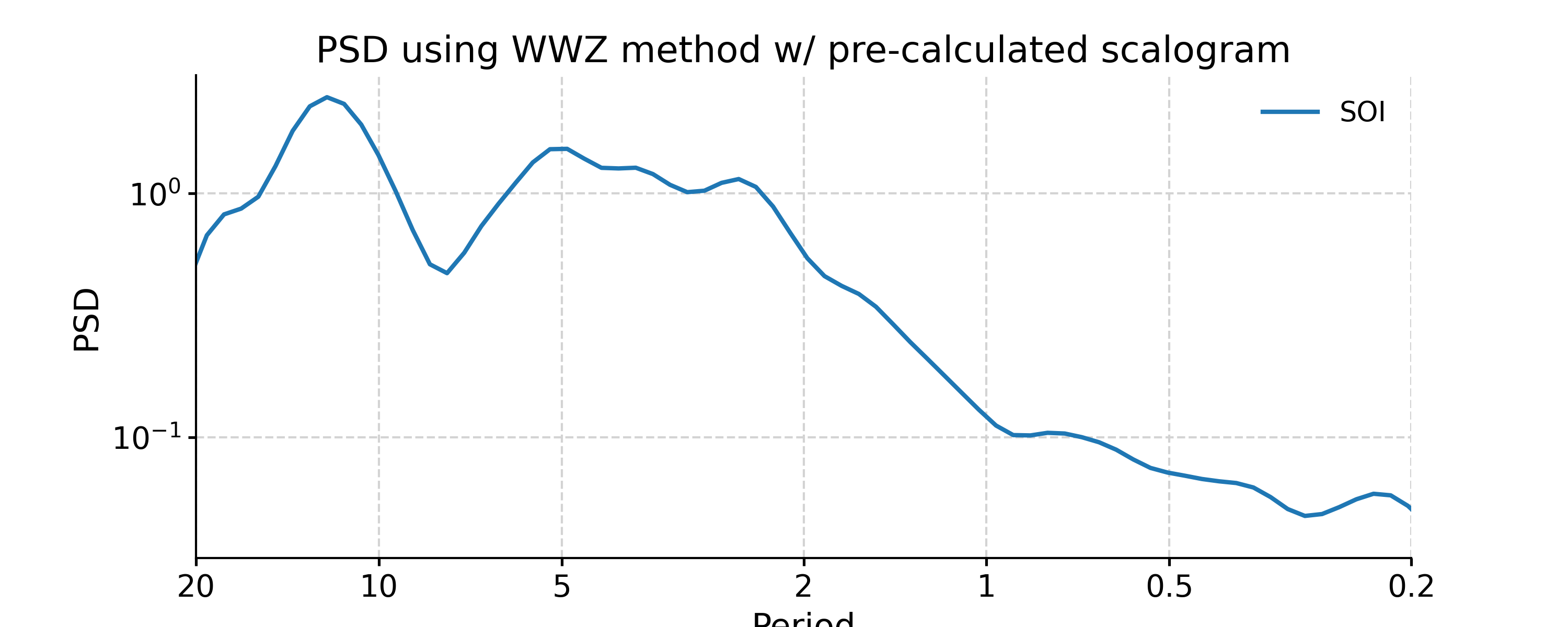
We may take advantage of a pre-calculated scalogram using WWZ to accelerate the spectral analysis (although note that the default parameters for spectral and wavelet analysis using WWZ are different):

In [24]: scal_wwz = ts_std.wavelet(method='wwz')  # wwz is the default method

In [25]: psd_wwz_fast = ts_std.spectral(method='wwz', scalogram=scal_wwz)

In [26]: fig, ax = psd_wwz_fast.plot(title='PSD using WWZ method w/ pre-calculated scalogram')

In [27]: pyleo.closefig(fig)

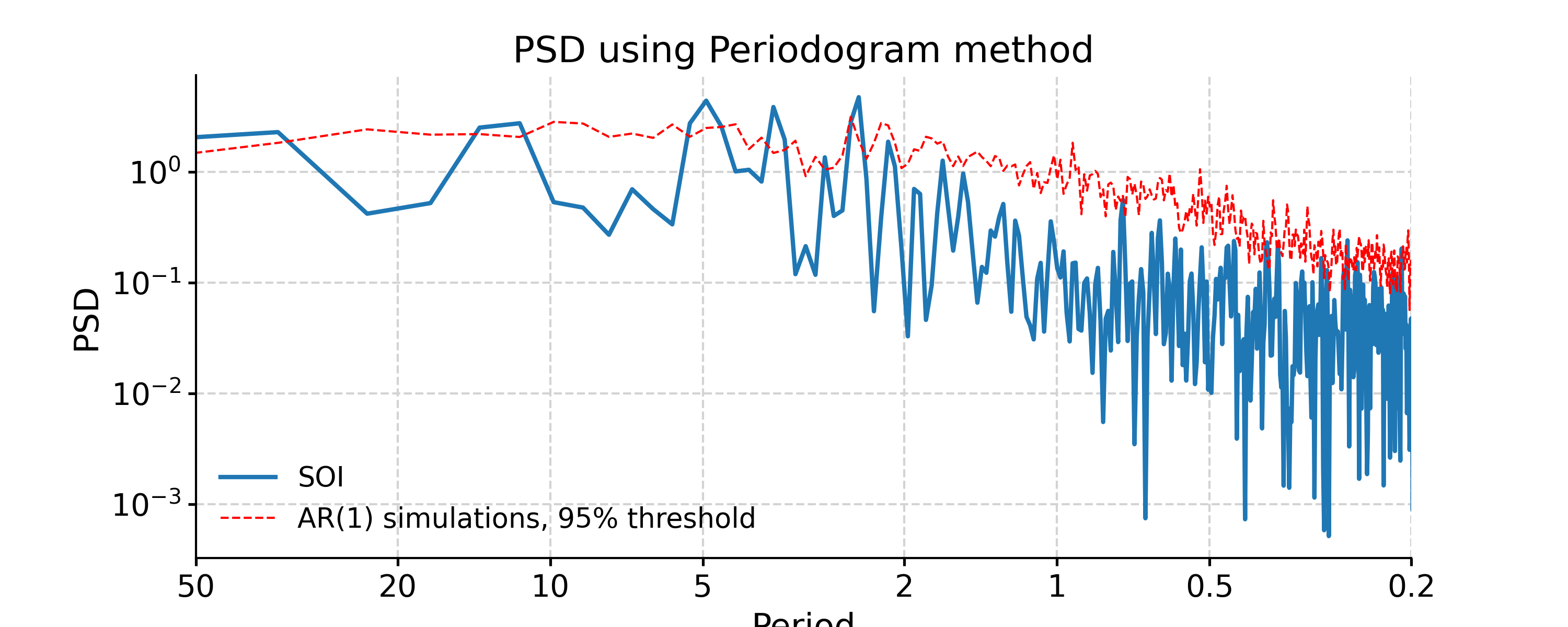
Periodogram

In [28]: ts_interp = ts_std.interp()

In [29]: psd_perio = ts_interp.spectral(method='periodogram')

In [30]: psd_perio_signif = psd_perio.signif_test(number=20, method='ar1sim') #in practice, need more AR1 simulations

In [31]: fig, ax = psd_perio_signif.plot(title='PSD using Periodogram method')

In [32]: pyleo.closefig(fig)

Welch

In [33]: psd_welch = ts_interp.spectral(method='welch')

In [34]: psd_welch_signif = psd_welch.signif_test(number=20, method='ar1sim') #in practice, need more AR1 simulations

In [35]: fig, ax = psd_welch_signif.plot(title='PSD using Welch method')

In [36]: pyleo.closefig(fig)

MTM

In [37]: psd_mtm = ts_interp.spectral(method='mtm', label='MTM, NW=4')

In [38]: psd_mtm_signif = psd_mtm.signif_test(number=20, method='ar1sim') #in practice, need more AR1 simulations

In [39]: fig, ax = psd_mtm_signif.plot(title='PSD using the multitaper method')

In [40]: pyleo.closefig(fig)

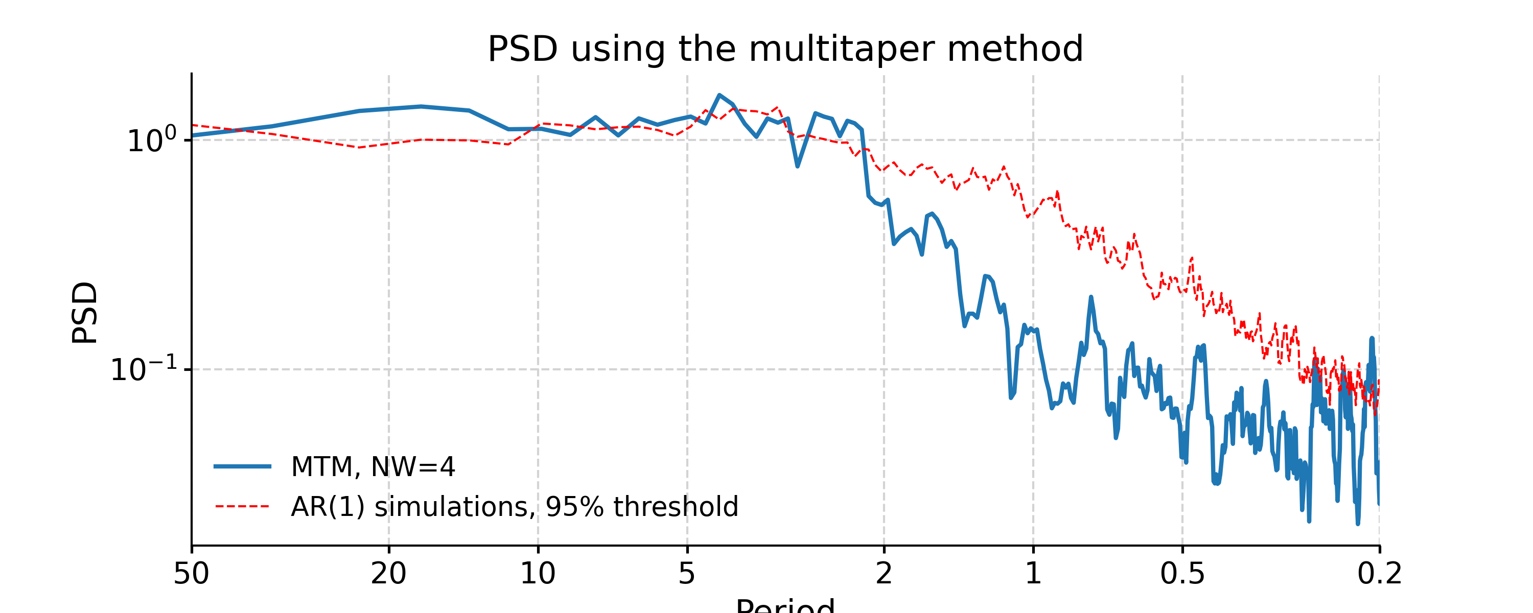
By default, MTM uses a half-bandwidth of 4 times the fundamental (Rayleigh) frequency, i.e. NW = 4, which is the most conservative choice. NW runs from 2 to 4 in multiples of 1/2, and can be adjusted like so (note the sharper peaks and higher overall variance, which may not be desirable):

In [41]: psd_mtm2 = ts_interp.spectral(method='mtm', settings={'NW':2}, label='MTM, NW=2')

In [42]: psd_mtm2.plot(title='PSD using the multi-taper method', ax=ax)
Out[42]: <AxesSubplot: title={'center': 'PSD using the multi-taper method'}, xlabel='Period', ylabel='PSD'>

In [43]: pyleo.closefig(fig)

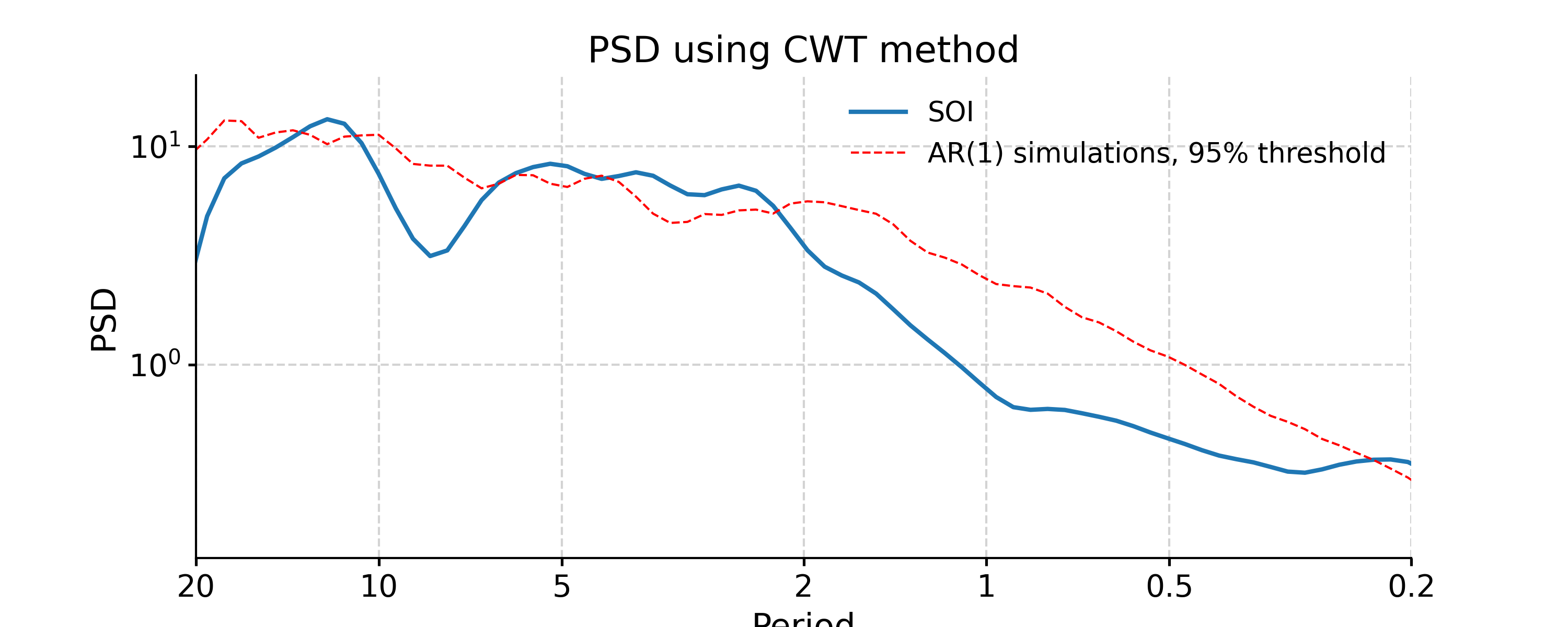
Continuous Wavelet Transform

In [44]: ts_interp = ts_std.interp()

In [45]: psd_cwt = ts_interp.spectral(method='cwt')

In [46]: psd_cwt_signif = psd_cwt.signif_test(number=20)

In [47]: fig, ax = psd_cwt_signif.plot(title='PSD using CWT method')

In [48]: pyleo.closefig(fig)

ssa(M=None, nMC=0, f=0.3, trunc=None, var_thresh=80)[source]

Singular Spectrum Analysis

Nonparametric, orthogonal decomposition of timeseries into constituent oscillations. This implementation uses the method of [1], with applications presented in [2]. Optionally (MC>0), the significance of eigenvalues is assessed by Monte-Carlo simulations of an AR(1) model fit to X, using [3]. The method expects regular spacing, but is tolerant to missing values, up to a fraction 0<f<1 (see [4]).

Parameters:

M (int, optional) – window size. The default is None (10% of the length of the series).
MC (int, optional) – Number of iteration in the Monte-Carlo process. The default is 0.
f (float, optional) – maximum allowable fraction of missing values. The default is 0.3.
trunc (str) –
if present, truncates the expansion to a level K < M owing to one of 3 criteria:
1. ’kaiser’: variant of the Kaiser-Guttman rule, retaining eigenvalues larger than the median
2. ’mcssa’: Monte-Carlo SSA (use modes above the 95% threshold)
3. ’var’: first K modes that explain at least var_thresh % of the variance.
Default is None, which bypasses truncation (K = M)
var_thresh (float) – variance threshold for reconstruction (only impactful if trunc is set to ‘var’)

Returns:

res (object of the SsaRes class containing:)
eigvals ((M, ) array of eigenvalues)
eigvecs ((M, M) Matrix of temporal eigenvectors (T-EOFs))
PC ((N - M + 1, M) array of principal components (T-PCs))
RCmat ((N, M) array of reconstructed components)
RCseries ((N,) reconstructed series, with mean and variance restored)
pctvar ((M, ) array of the fraction of variance (%) associated with each mode)
eigvals_q ((M, 2) array contaitning the 5% and 95% quantiles of the Monte-Carlo eigenvalue spectrum [ if nMC >0 ])

References

[1]_ Vautard, R., and M. Ghil (1989), Singular spectrum analysis in nonlinear dynamics, with applications to paleoclimatic time series, Physica D, 35, 395–424.

[2]_ Ghil, M., R. M. Allen, M. D. Dettinger, K. Ide, D. Kondrashov, M. E. Mann, A. Robertson, A. Saunders, Y. Tian, F. Varadi, and P. Yiou (2002), Advanced spectral methods for climatic time series, Rev. Geophys., 40(1), 1003–1052, doi:10.1029/2000RG000092.

[3]_ Allen, M. R., and L. A. Smith (1996), Monte Carlo SSA: Detecting irregular oscillations in the presence of coloured noise, J. Clim., 9, 3373–3404.

[4]_ Schoellhamer, D. H. (2001), Singular spectrum analysis for time series with missing data, Geophysical Research Letters, 28(16), 3187–3190, doi:10.1029/2000GL012698.

See also

pyleoclim.core.utils.decomposition.ssa: Singular Spectrum Analysis utility
pyleoclim.core.ssares.SsaRes.modeplot: plot SSA modes
pyleoclim.core.ssares.SsaRes.screeplot: plot SSA eigenvalue spectrum

Examples

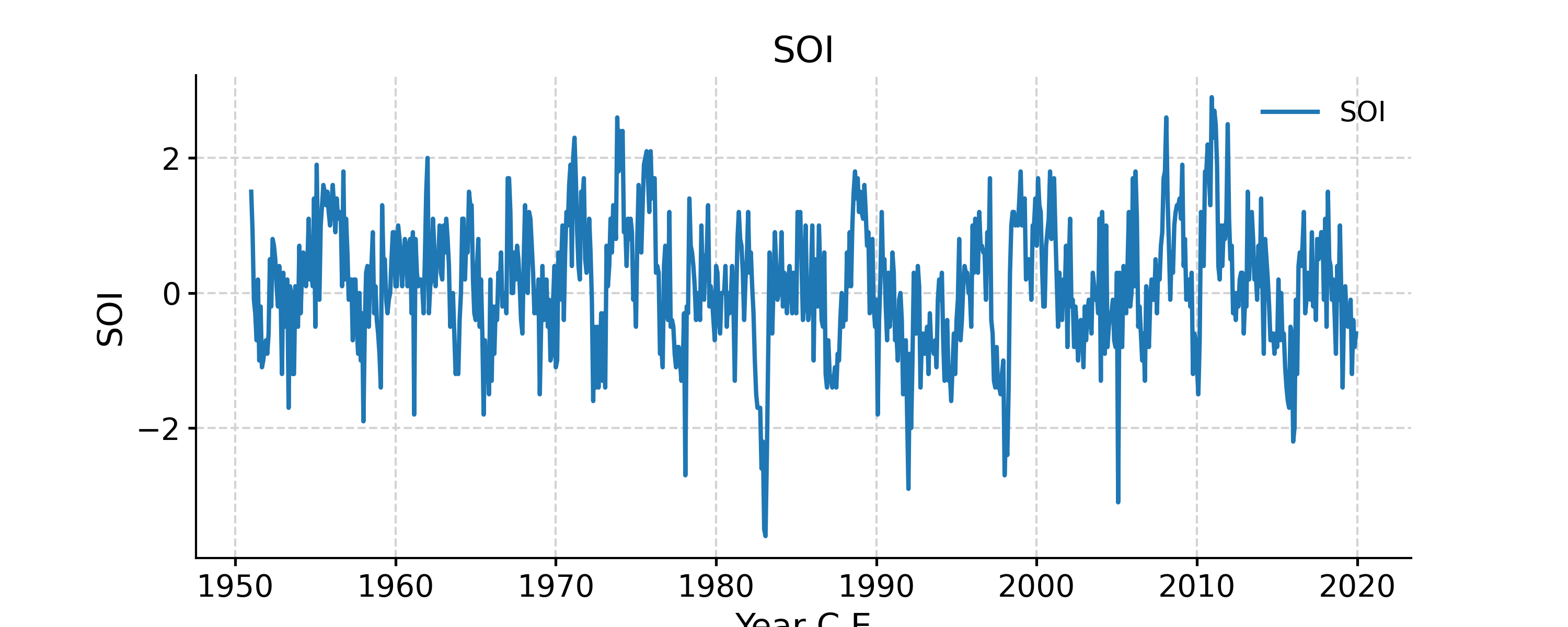
SSA with SOI

In [1]: import pyleoclim as pyleo

In [2]: import pandas as pd

In [3]: data = pd.read_csv('https://raw.githubusercontent.com/LinkedEarth/Pyleoclim_util/Development/example_data/soi_data.csv',skiprows=0,header=1)

In [4]: time = data.iloc[:,1]

In [5]: value = data.iloc[:,2]

In [6]: ts = pyleo.Series(time=time, value=value, time_name='Year C.E', value_name='SOI', label='SOI')

In [7]: fig, ax = ts.plot()

In [8]: pyleo.closefig(fig)

In [9]: nino_ssa = ts.ssa(M=60)

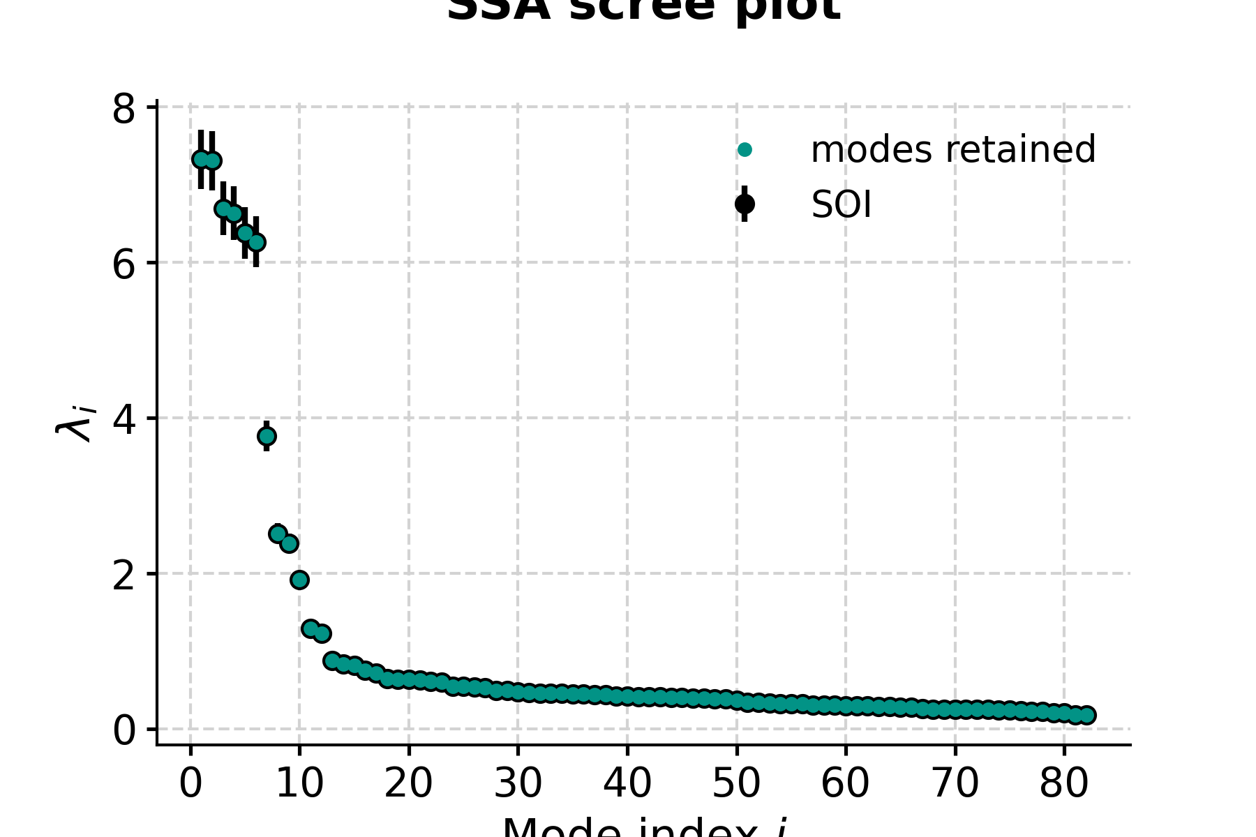
Let us now see how to make use of all these arrays. The first step is too inspect the eigenvalue spectrum (“scree plot”) to identify remarkable modes. Let us restrict ourselves to the first 40, so we can see something:

In [10]: fig, ax = nino_ssa.screeplot()

In [11]: pyleo.closefig(fig)

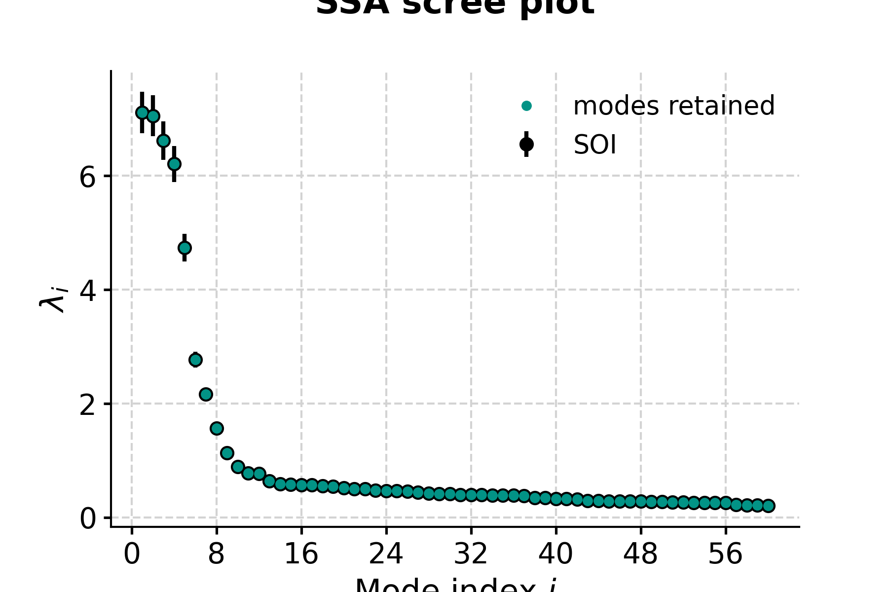
This highlights a few common phenomena with SSA:

the eigenvalues are in descending order
their uncertainties are proportional to the eigenvalues themselves
the eigenvalues tend to come in pairs : (1,2) (3,4), are all clustered within uncertainties . (5,6) looks like another doublet
around i=15, the eigenvalues appear to reach a floor, and all subsequent eigenvalues explain a very small amount of variance.

So, summing the variance of the first 15 modes, we get:

In [12]: print(nino_ssa.pctvar[:14].sum())
97.03202170599148

That is a typical result for a (paleo)climate timeseries; a few modes do the vast majority of the work. That means we can focus our attention on these modes and capture most of the interesting behavior. To see this, let’s use the reconstructed components (RCs), and sum the RC matrix over the first 15 columns:

In [13]: RCk = nino_ssa.RCmat[:,:14].sum(axis=1)

In [14]: fig, ax = ts.plot(title='SOI')

In [15]: ax.plot(time,RCk,label='SSA reconstruction, 14 modes',color='orange')
Out[15]: [<matplotlib.lines.Line2D at 0x7f17eb93ae60>]

In [16]: ax.legend()
Out[16]: <matplotlib.legend.Legend at 0x7f17e9c3c310>

In [17]: pyleo.closefig(fig)

Indeed, these first few modes capture the vast majority of the low-frequency behavior, including all the El Niño/La Niña events. What is left (the blue wiggles not captured in the orange curve) are high-frequency oscillations that might be considered “noise” from the standpoint of ENSO dynamics. This illustrates how SSA might be used for filtering a timeseries. One must be careful however:

there was not much rhyme or reason for picking 14 modes. Why not 5, or 39? All we have seen so far is that they gather >95% of the variance, which is by no means a magic number.
there is no guarantee that the first few modes will filter out high-frequency behavior, or at what frequency cutoff they will do so. If you need to cut out specific frequencies, you are better off doing it with a classical filter, like the butterworth filter implemented in Pyleoclim. However, in many instances the choice of a cutoff frequency is itself rather arbitrary. In such cases, SSA provides a principled alternative for generating a version of a timeseries that preserves features and excludes others (i.e, a filter).
as with all orthgonal decompositions, summing over all RCs will recover the original signal within numerical precision.

Monte-Carlo SSA

Selecting meaningful modes in eigenproblems (e.g. EOF analysis) is more art than science. However, one technique stands out: Monte Carlo SSA, introduced by Allen & Smith, (1996) to identify SSA modes that rise above what one would expect from “red noise”, specifically an AR(1) process). To run it, simply provide the parameter MC, ideally with a number of iterations sufficient to get decent statistics. Here let’s use MC = 1000. The result will be stored in the eigval_q array, which has the same length as eigval, and its two columns contain the 5% and 95% quantiles of the ensemble of MC-SSA eigenvalues.

In [18]: nino_mcssa = ts.ssa(M = 60, nMC=1000)

Now let’s look at the result:

In [19]: fig, ax = nino_mcssa.screeplot()

In [20]: pyleo.closefig(fig)

In [21]: print('Indices of modes retained: '+ str(nino_mcssa.mode_idx))
Indices of modes retained: [ 0  1  2  3  4 14 20 25 27 28 29 30]

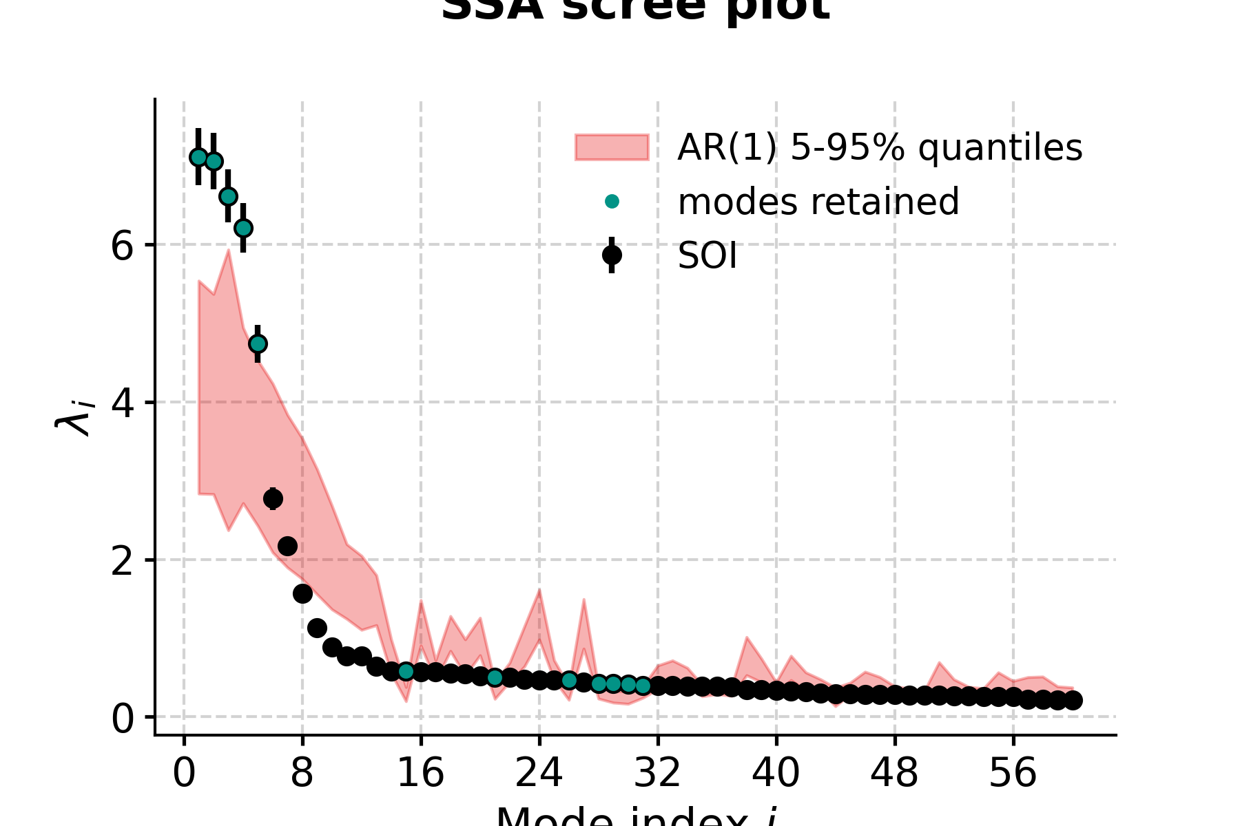
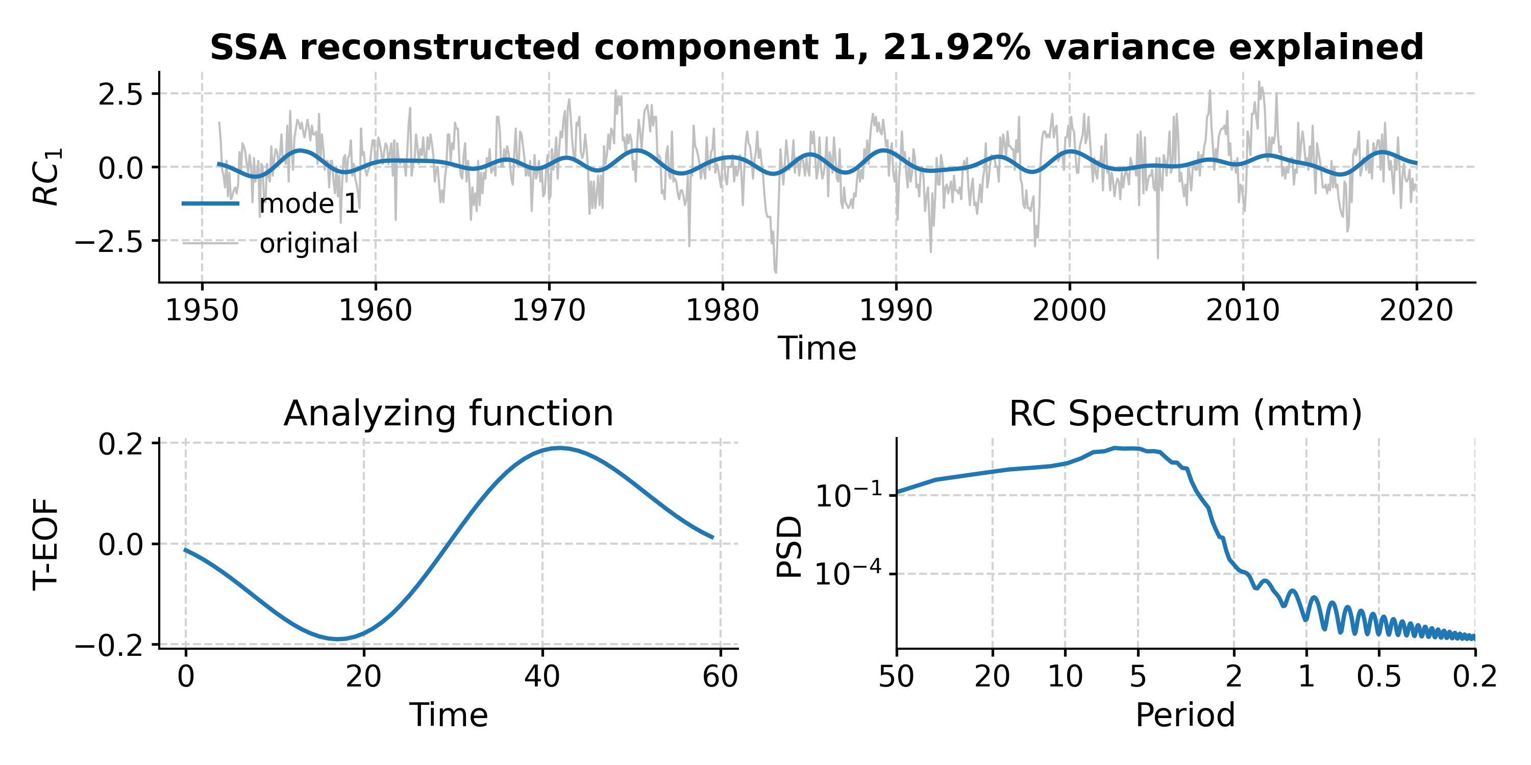
This suggests that modes 1-5 fall above the red noise benchmark. To inspect mode 1 (index 0), just type:

In [22]: fig, ax = nino_mcssa.modeplot(index=0)

In [23]: pyleo.closefig(fig)

standardize(keep_log=False, scale=1)[source]

Standardizes the series ((i.e. remove its estimated mean and divides by its estimated standard deviation)

Returns:

new (Series) – The standardized series object
keep_log (Boolean) – if True, adds the previous mean, standard deviation and method parameters to the series log.

stats()[source]

Compute basic statistics from a Series

Computes the mean, median, min, max, standard deviation, and interquartile range of a numpy array y, ignoring NaNs.

Returns:: res – Contains the mean, median, minimum value, maximum value, standard deviation, and interquartile range for the Series.
Return type:: dictionary

Examples

Compute basic statistics for the SOI series

In [1]: import pyleoclim as pyleo

In [2]: import pandas as pd

In [3]: data=pd.read_csv('https://raw.githubusercontent.com/LinkedEarth/Pyleoclim_util/Development/example_data/soi_data.csv',skiprows=0,header=1)

In [4]: time=data.iloc[:,1]

In [5]: value=data.iloc[:,2]

In [6]: ts=pyleo.Series(time=time,value=value,time_name='Year C.E', value_name='SOI', label='SOI')

In [7]: ts.stats()
Out[7]: 
{'mean': 0.11992753623188407,
 'median': 0.1,
 'min': -3.6,
 'max': 2.9,
 'std': 0.9380195472790024,
 'IQR': 1.3}

stripes(ref_period, LIM=2.8, thickness=1.0, figsize=[8, 1], xlim=None, top_label=None, bottom_label=None, label_color='gray', label_size=None, xlabel=None, savefig_settings=None, ax=None, invert_xaxis=False, show_xaxis=False, x_offset=0.05)[source]

Represents the Series as an Ed Hawkins “stripes” pattern

Credit: https://matplotlib.org/matplotblog/posts/warming-stripes/

Parameters:

ref_period (array-like (2-elements)) – dates of the reference period, in the form “(first, last)”
thickness (float, optional) – vertical thickness of the stripe . The default is 1.0
LIM (float) – scaling factor for color saturation. default is 2.8
figsize (list) – a list of two integers indicating the figure size (in inches)
xlim (list) – time axis limits
top_label (str) – the “title” label for the stripe
bottom_label (str) – the “ylabel” explaining which variable is being plotted
invert_xaxis (bool, optional) – if True, the x-axis of the plot will be inverted
x_offset (float) – value controlling the horizontal offset between stripes and labels (default = 0.05)
show_xaxis (bool) – flag indicating whether or not the x-axis should be shown (default = False)
savefig_settings (dict) –
the dictionary of arguments for plt.savefig(); some notes below: - “path” must be specified; it can be any existed or non-existed path,

with or without a suffix; if the suffix is not given in “path”, it will follow “format”
- ”format” can be one of {“pdf”, “eps”, “png”, “ps”}
ax (matplotlib.axis, optional) – the axis object from matplotlib See [matplotlib.axes](https://matplotlib.org/api/axes_api.html) for details.

Returns:

fig (matplotlib.figure) – the figure object from matplotlib See [matplotlib.pyplot.figure](https://matplotlib.org/stable/api/figure_api.html) for details.
ax (matplotlib.axis) – the axis object from matplotlib See [matplotlib.axes](https://matplotlib.org/stable/api/axes_api.html) for details.

Notes

When ax is passed, the return will be ax only; otherwise, both fig and ax will be returned.

See also

pyleoclim.utils.plotting.stripes: stripes representation of a timeseries
pyleoclim.utils.plotting.savefig: saving a figure in Pyleoclim

Examples

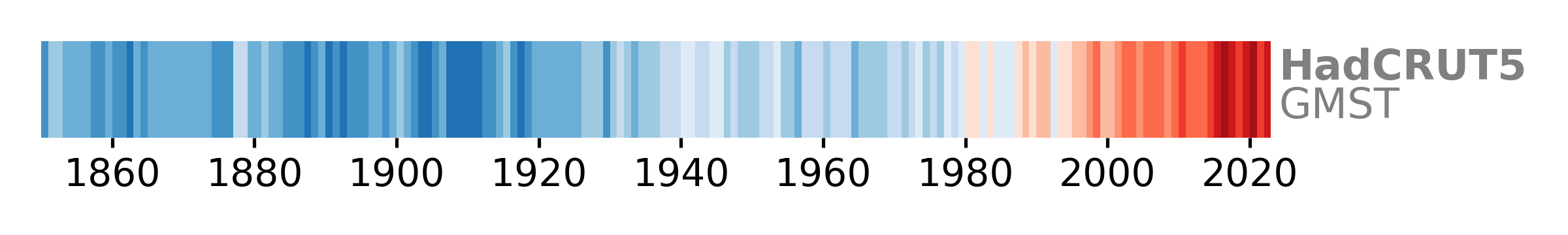
Plot the HadCRUT5 Global Mean Surface Temperature

In [1]: import pyleoclim as pyleo

In [2]: import pandas as pd

In [3]: url = 'https://www.metoffice.gov.uk/hadobs/hadcrut5/data/current/analysis/diagnostics/HadCRUT.5.0.1.0.analysis.summary_series.global.annual.csv'

In [4]: df = pd.read_csv(url)

In [5]: time = df['Time']

In [6]: gmst = df['Anomaly (deg C)']

In [7]: ts = pyleo.Series(time=time,value=gmst, label = 'HadCRUT5', time_name='Year C.E', value_name='GMST')

In [8]: fig, ax = ts.stripes(ref_period=(1971,2000))

In [9]: pyleo.closefig(fig)

If you wanted to show the time axis:

In [10]: import pyleoclim as pyleo

In [11]: import pandas as pd

In [12]: url = 'https://www.metoffice.gov.uk/hadobs/hadcrut5/data/current/analysis/diagnostics/HadCRUT.5.0.1.0.analysis.summary_series.global.annual.csv'

In [13]: df = pd.read_csv(url)

In [14]: time = df['Time']

In [15]: gmst = df['Anomaly (deg C)']

In [16]: ts = pyleo.Series(time=time,value=gmst, label = 'HadCRUT5', time_name='Year C.E', value_name='GMST')

In [17]: fig, ax = ts.stripes(ref_period=(1971,2000), show_xaxis=True, figsize=[8, 1.2])

In [18]: pyleo.closefig(fig)

Note that we had to increase the figure height to make space for the extra text.

summary_plot(psd, scalogram, figsize=[8, 10], title=None, time_lim=None, value_lim=None, period_lim=None, psd_lim=None, time_label=None, value_label=None, period_label=None, psd_label=None, ts_plot_kwargs=None, wavelet_plot_kwargs=None, psd_plot_kwargs=None, gridspec_kwargs=None, y_label_loc=None, legend=None, savefig_settings=None)[source]

Produce summary plot of timeseries.

Generate cohesive plot of timeseries alongside results of wavelet analysis and spectral analysis on said timeseries. Requires wavelet and spectral analysis to be conducted outside of plotting function, psd and scalogram must be passed as arguments.

Parameters:

psdPSD

the PSD object of a Series.

scalogramScalogram

the Scalogram object of a Series. If the passed scalogram object contains stored signif_scals these will be plotted.

figsizelist

a list of two integers indicating the figure size

titlestr

the title for the figure

time_limlist or tuple

the limitation of the time axis. This is for display purposes only, the scalogram and psd will still be calculated using the full time series.

value_limlist or tuple

the limitation of the value axis of the timeseries. This is for display purposes only, the scalogram and psd will still be calculated using the full time series.

period_limlist or tuple

the limitation of the period axis

psd_limlist or tuple

the limitation of the psd axis

time_labelstr

the label for the time axis

value_labelstr

the label for the value axis of the timeseries

period_labelstr

the label for the period axis

psd_labelstr

the label for the amplitude axis of PDS

legendbool

if set to True, a legend will be added to the open space above the psd plot

ts_plot_kwargsdict

arguments to be passed to the timeseries subplot, see Series.plot for details

wavelet_plot_kwargsdict

arguments to be passed to the scalogram plot, see pyleoclim.Scalogram.plot for details

psd_plot_kwargsdict

arguments to be passed to the psd plot, see PSD.plot for details Certain psd plot settings are required by summary plot formatting. These include:

ylabel

legend

tick parameters

These will be overriden by summary plot to prevent formatting errors

gridspec_kwargsdict

arguments used to build the specifications for gridspec configuration The plot is constructed with six slots:

slot [0] contains a subgridspec containing the timeseries and scalogram (shared x axis)

slot [1] contains a subgridspec containing an empty slot and the PSD plot (shared y axis with scalogram)

slot [2] and slot [3] are empty to allow ample room for xlabels for the scalogram and PSD plots

slot [4] contains the scalogram color bar

slot [5] is empty

It is possible to tune the size and spacing of the various slots

‘width_ratios’: list of two values describing the relative widths of the two columns (default: [6, 1])
‘height_ratios’: list of three values describing the relative heights of the three rows (default: [2, 7, .35])
‘hspace’: vertical space between timeseries and scalogram (default: 0, however if either the scalogram xlabel or the PSD xlabel contain ‘

‘, .05)

‘wspace’: lateral space between scalogram and psd plot slots (default: 0.05)

‘cbspace’: vertical space between the scalogram and colorbar

y_label_locfloat

Plot parameter to adjust horizontal location of y labels to avoid conflict with axis labels, default value is -0.15

savefig_settingsdict

the dictionary of arguments for plt.savefig(); some notes below: - “path” must be specified; it can be any existed or non-existed path,

with or without a suffix; if the suffix is not given in “path”, it will follow “format”

“format” can be one of {“pdf”, “eps”, “png”, “ps”}

See also

pyleoclim.core.series.Series.spectral: Spectral analysis for a timeseries
pyleoclim.core.series.Series.wavelet: Wavelet analysis for a timeseries
pyleoclim.utils.plotting.savefig: saving figure in Pyleoclim
pyleoclim.core.psds.PSD: PSD object
pyleoclim.core.psds.MultiplePSD: Multiple PSD object

Examples

Summary_plot with pre-generated psd and scalogram objects. Note that if the scalogram contains saved noise realizations these will be flexibly reused. See pyleo.Scalogram.signif_test() for details

In [1]: import pyleoclim as pyleo

In [2]: import pandas as pd

In [3]: ts=pd.read_csv('https://raw.githubusercontent.com/LinkedEarth/Pyleoclim_util/master/example_data/soi_data.csv',skiprows = 1)

In [4]: series = pyleo.Series(time = ts['Year'],value = ts['Value'], time_name = 'Years', time_unit = 'AD')

In [5]: psd = series.spectral(freq_method = 'welch')

In [6]: scalogram = series.wavelet(freq_method = 'welch')

In [7]: fig, ax = series.summary_plot(psd = psd,scalogram = scalogram)

In [8]: pyleo.closefig(fig)

Summary_plot with pre-generated psd and scalogram objects from before and some plot modification arguments passed. Note that if the scalogram contains saved noise realizations these will be flexibly reused. See pyleo.Scalogram.signif_test() for details

In [9]: import pyleoclim as pyleo

In [10]: import pandas as pd

In [11]: ts=pd.read_csv('https://raw.githubusercontent.com/LinkedEarth/Pyleoclim_util/master/example_data/soi_data.csv',skiprows = 1)

In [12]: series = pyleo.Series(time = ts['Year'],value = ts['Value'], time_name = 'Years', time_unit = 'AD')

In [13]: psd = series.spectral(freq_method = 'welch')

In [14]: scalogram = series.wavelet(freq_method = 'welch')

In [15]: fig, ax = series.summary_plot(psd = psd,scalogram = scalogram, period_lim = [5,0], ts_plot_kwargs = {'color':'red','linewidth':.5}, psd_plot_kwargs = {'color':'red','linewidth':.5})

In [16]: pyleo.closefig(fig)

surrogates(method='ar1sim', number=1, length=None, seed=None, settings=None)[source]

Generate surrogates with increasing time axis

Parameters:

method ({ar1sim}) – Uses an AR1 model to generate surrogates of the timeseries
number (int) – The number of surrogates to generate
length (int) – Length of the series
seed (int) – Control seed option for reproducibility
settings (dict) – Parameters for surogate generator. See individual methods for details.

Returns:

surr

Return type:

SurrogateSeries

See also

pyleoclim.utils.tsmodel.ar1_sim: AR(1) simulator

wavelet(method='cwt', settings=None, freq_method='log', freq_kwargs=None, verbose=False)[source]

Perform wavelet analysis on a timeseries

Parameters:

method (str {wwz, cwt}) –

cwt - the continuous wavelet transform [1]
is appropriate for evenly-spaced series.

wwz - the weighted wavelet Z-transform [2]
is appropriate for unevenly-spaced series.

Default is cwt, returning an error if the Series is unevenly-spaced.
freq_method (str) – {‘log’, ‘scale’, ‘nfft’, ‘lomb_scargle’, ‘welch’}
freq_kwargs (dict) – Arguments for the frequency vector
settings (dict) – Arguments for the specific wavelet method
verbose (bool) – If True, will print warning messages if there is any

Returns:

scal

Return type:

Scalogram object

See also

pyleoclim.utils.wavelet.wwz: wwz function
pyleoclim.utils.wavelet.cwt: cwt function
pyleoclim.utils.spectral.make_freq_vector: Functions to create the frequency vector
pyleoclim.utils.tsutils.detrend: Detrending function
pyleoclim.core.series.Series.spectral: spectral analysis tools
pyleoclim.core.scalograms.Scalogram: Scalogram object
pyleoclim.core.scalograms.MultipleScalogram: Multiple Scalogram object

References

[1] Torrence, C. and G. P. Compo, 1998: A Practical Guide to Wavelet Analysis. Bull. Amer. Meteor. Soc., 79, 61-78. Python routines available at http://paos.colorado.edu/research/wavelets/

[2] Foster, G., 1996: Wavelets for period analysis of unevenly sampled time series. The Astronomical Journal, 112, 1709.

Examples

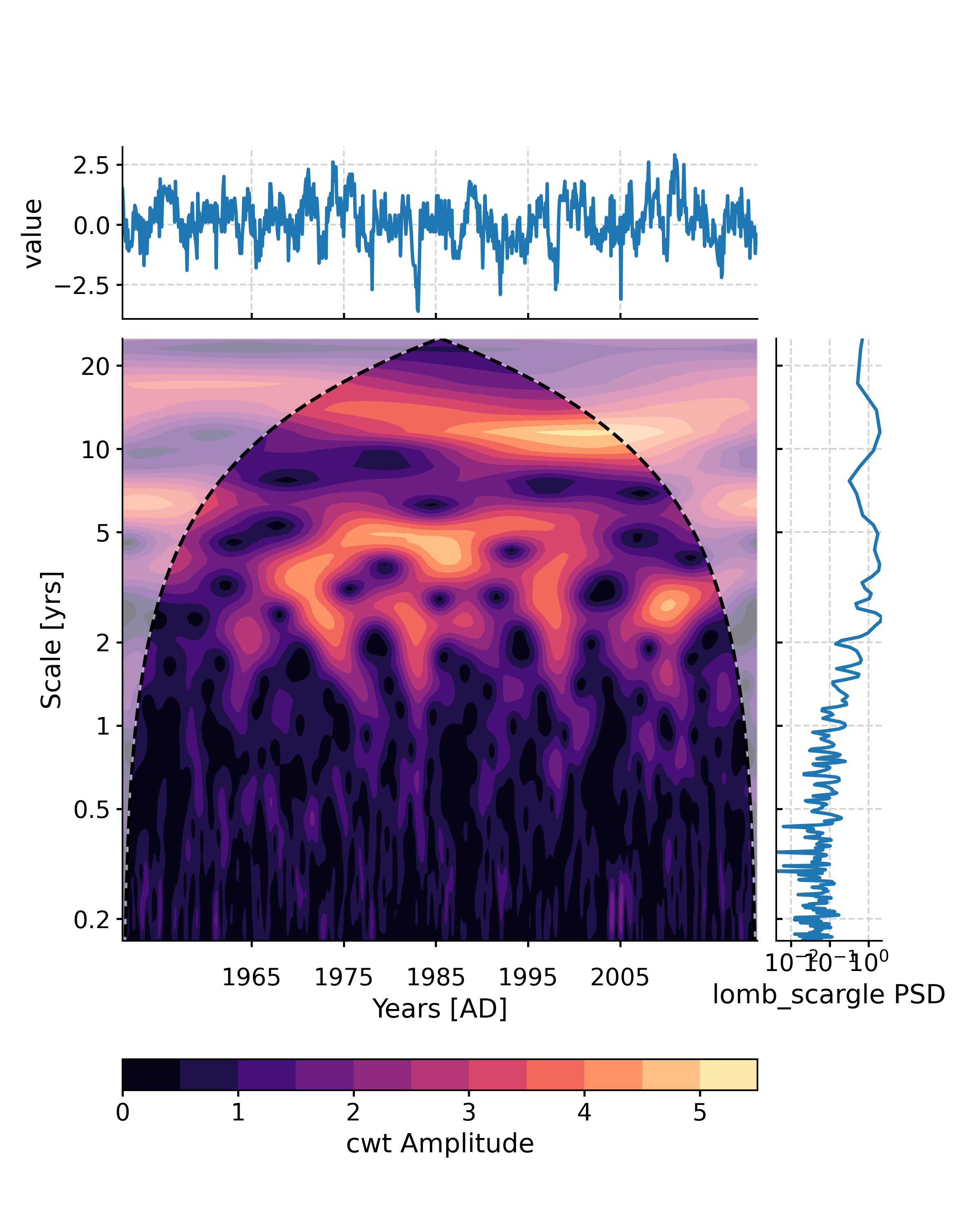
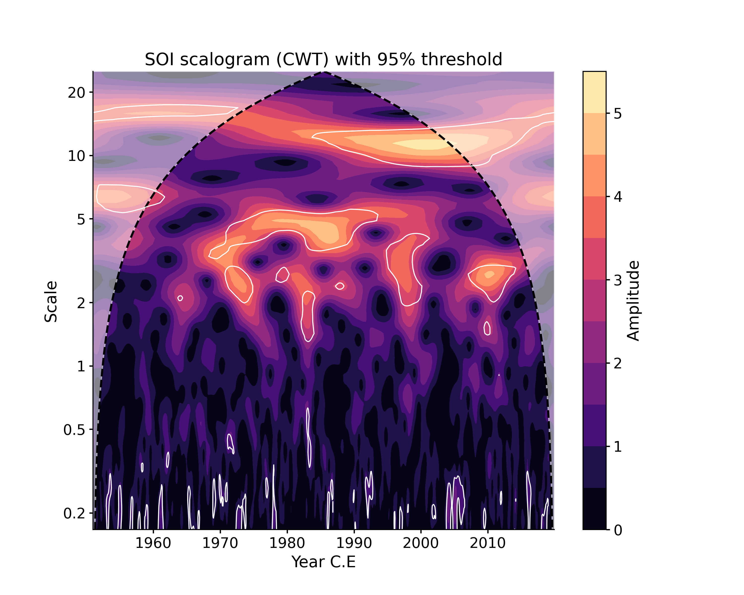
Wavelet analysis on the evenly-spaced SOI record. The CWT method will be applied by default.

In [1]: import pyleoclim as pyleo

In [2]: import pandas as pd

In [3]: data = pd.read_csv('https://raw.githubusercontent.com/LinkedEarth/Pyleoclim_util/Development/example_data/soi_data.csv',skiprows=0,header=1)

In [4]: time = data.iloc[:,1]

In [5]: value = data.iloc[:,2]

In [6]: ts = pyleo.Series(time=time,value=value,time_name='Year C.E', value_name='SOI', label='SOI')

In [7]: scal1 = ts.wavelet()

In [8]: scal_signif = scal1.signif_test(number=20)  # for research-grade work, use number=200 or larger

In [9]: fig, ax = scal_signif.plot()

In [10]: pyleo.closefig(fig)

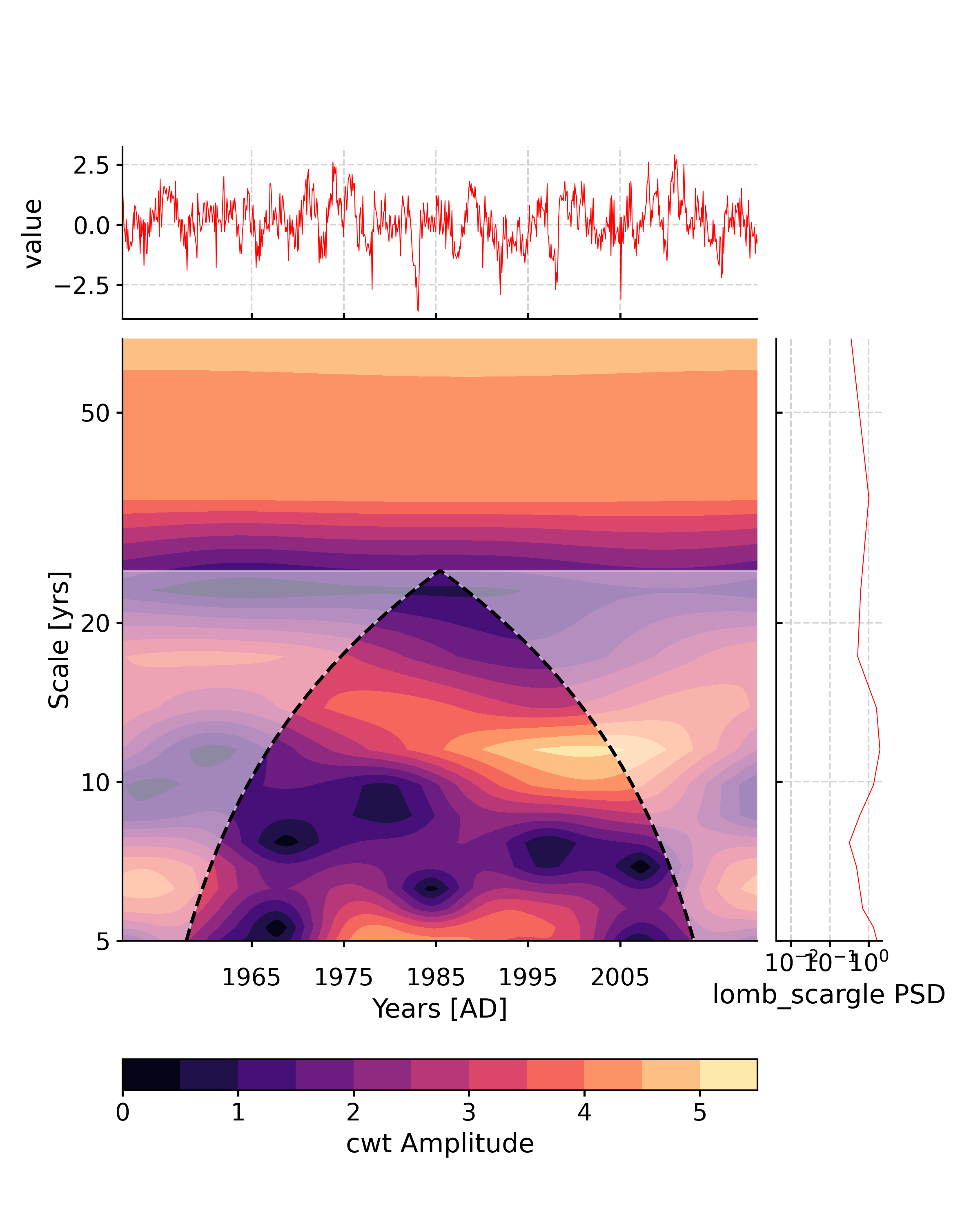
If you wanted to invoke the WWZ method instead (here with no significance testing, to lower computational cost):

In [11]: scal2 = ts.wavelet(method='wwz')

In [12]: fig, ax = scal2.plot()

In [13]: pyleo.closefig(fig)

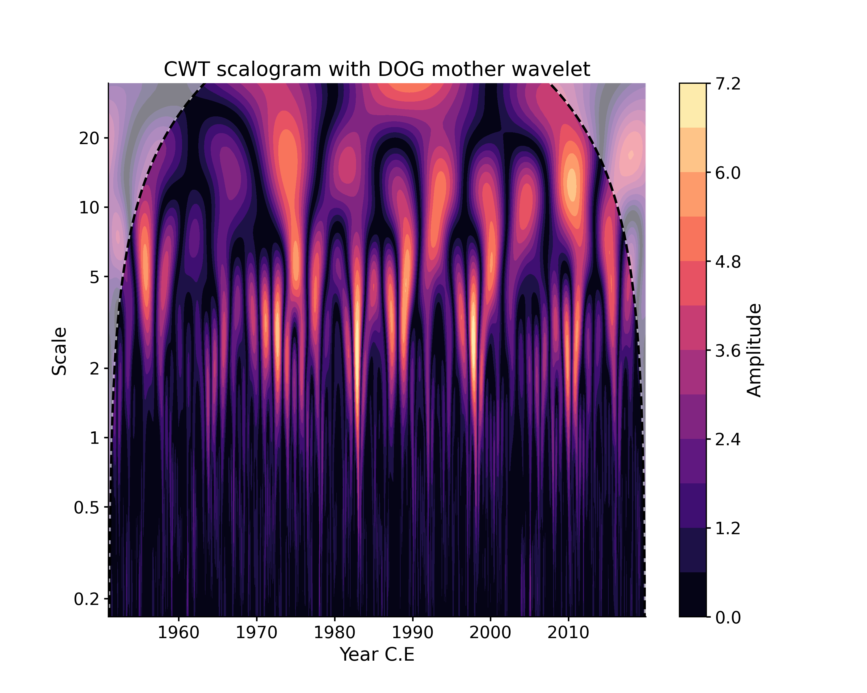
Notice that the two scalograms have different amplitude, which are relative. Method-specific arguments may be passed via settings. For instance, if you wanted to change the default mother wavelet (‘MORLET’) to a derivative of a Gaussian (DOG), with degree 2 by default (“Mexican Hat wavelet”):

In [14]: scal3 = ts.wavelet(settings = {'mother':'DOG'})

In [15]: fig, ax = scal3.plot(title='CWT scalogram with DOG mother wavelet')

In [16]: pyleo.closefig(fig)

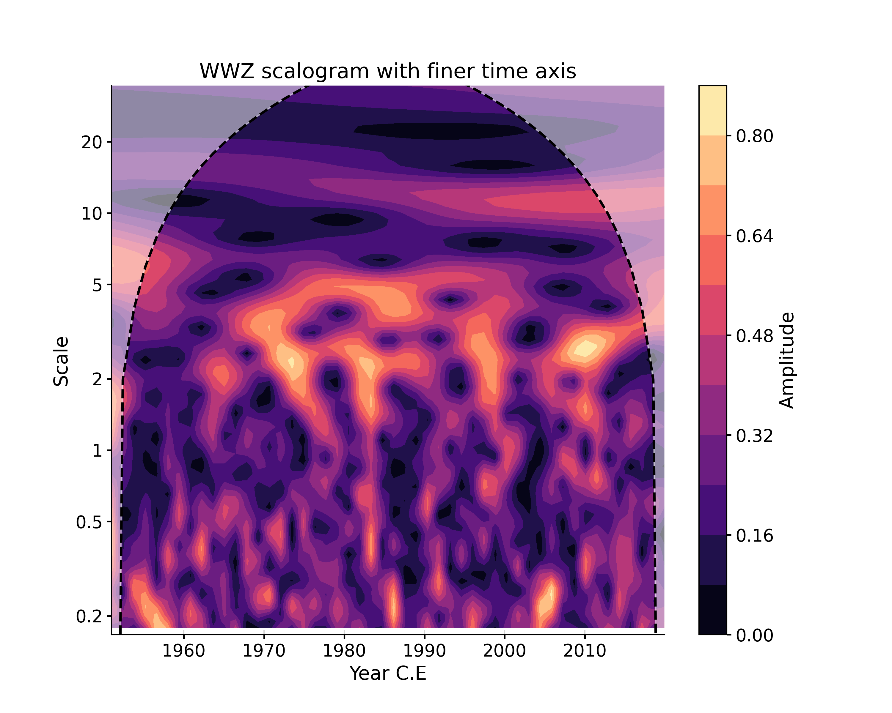
As for WWZ, note that, for computational efficiency, the time axis is coarse-grained by default to 50 time points, which explains in part the difference with the CWT scalogram.

If you need a custom axis, it (and other method-specific parameters) can also be passed via the settings dictionary:

In [17]: tau = np.linspace(np.min(ts.time), np.max(ts.time), 60)

In [18]: scal4 = ts.wavelet(method='wwz', settings={'tau':tau})

In [19]: fig, ax = scal4.plot(title='WWZ scalogram with finer time axis')

In [20]: pyleo.closefig(fig)

wavelet_coherence(target_series, method='cwt', settings=None, freq_method='log', freq_kwargs=None, verbose=False, common_time_kwargs=None)[source]

Performs wavelet coherence analysis with the target timeseries

Parameters:

target_series (Series) – A pyleoclim Series object on which to perform the coherence analysis
method (str) – Possible methods {‘wwz’,’cwt’}. Default is ‘cwt’, which only works if the series share the same evenly-spaced time axis. ‘wwz’ is designed for unevenly-spaced data, but is far slower.
freq_method (str) – {‘log’,’scale’, ‘nfft’, ‘lomb_scargle’, ‘welch’}
freq_kwargs (dict) – Arguments for frequency vector
common_time_kwargs (dict) – Parameters for the method MultipleSeries.common_time(). Will use interpolation by default.
settings (dict) – Arguments for the specific wavelet method (e.g. decay constant for WWZ, mother wavelet for CWT) and common properties like standardize, detrend, gaussianize, pad, etc.
verbose (bool) – If True, will print warning messages, if any

Returns:

coh

Return type:

pyleoclim.core.coherence.Coherence

References

Grinsted, A., Moore, J. C. & Jevrejeva, S. Application of the cross wavelet transform and wavelet coherence to geophysical time series. Nonlin. Processes Geophys. 11, 561–566 (2004).

See also

pyleoclim.utils.spectral.make_freq_vector: Functions to create the frequency vector
pyleoclim.utils.tsutils.detrend: Detrending function
pyleoclim.core.multipleseries.MultipleSeries.common_time: put timeseries on common time axis
pyleoclim.core.series.Series.wavelet: wavelet analysis
pyleoclim.utils.wavelet.wwz_coherence: coherence using the wwz method
pyleoclim.utils.wavelet.cwt_coherence: coherence using the cwt method

Examples

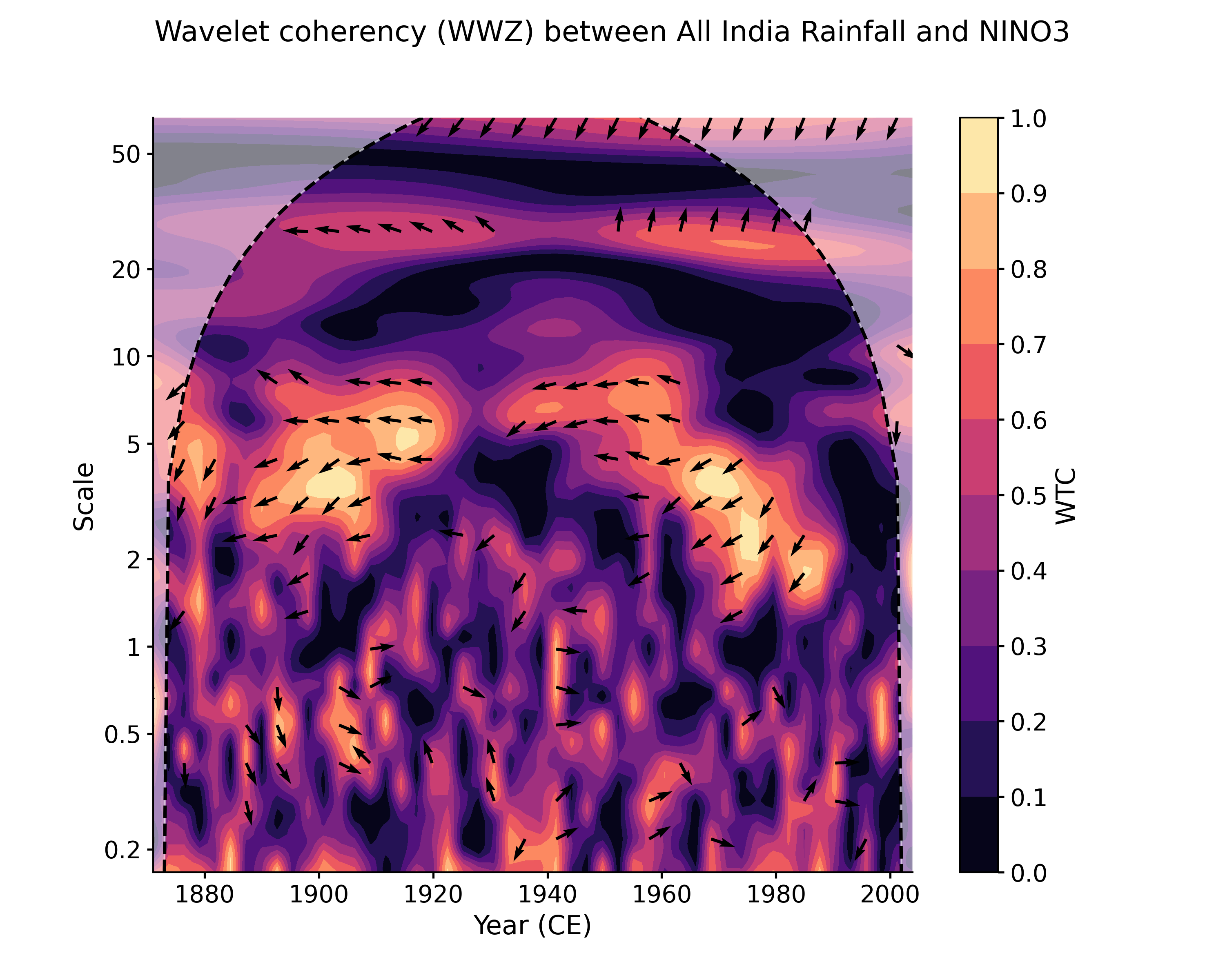
Calculate the wavelet coherence of NINO3 and All India Rainfall with default arguments:

In [1]: import pyleoclim as pyleo

In [2]: import pandas as pd

In [3]: data = pd.read_csv('https://raw.githubusercontent.com/LinkedEarth/Pyleoclim_util/Development/example_data/wtc_test_data_nino_even.csv')

In [4]: time = data['t'].values

In [5]: air = data['air'].values

In [6]: nino = data['nino'].values

In [7]: ts_air = pyleo.Series(time=time, value=data['air'].values, time_name='Year (CE)',
   ...:                       label='All India Rainfall', value_name='AIR (mm/month)')
   ...: 

In [8]: ts_nino = pyleo.Series(time=time, value=data['nino'].values, time_name='Year (CE)',
   ...:                        label='NINO3', value_name='NINO3 (K)')
   ...: 

In [9]: coh = ts_air.wavelet_coherence(ts_nino)

In [10]: coh.plot()
Out[10]: 
(<Figure size 1000x800 with 2 Axes>,
 <AxesSubplot: xlabel='Year (CE)', ylabel='Scale'>)

Note that in this example both timeseries area already on a common, evenly-spaced time axis. If they are not (either because the data are unevenly spaced, or because the time axes are different in some other way), an error will be raised. To circumvent this error, you can either put the series on a common time axis (e.g. using common_time()) prior to applying CWT, or you can use the Weighted Wavelet Z-transform (WWZ) instead, as it is designed for unevenly-spaced data. However, it is usually far slower:

In [11]: coh_wwz = ts_air.wavelet_coherence(ts_nino, method = 'wwz')

In [12]: coh_wwz.plot()
Out[12]: 
(<Figure size 1000x800 with 2 Axes>,
 <AxesSubplot: xlabel='Year (CE)', ylabel='Scale'>)

As with wavelet analysis, both CWT and WWZ admit optional arguments through settings. Significance is assessed similarly as with PSD or Scalogram objects:

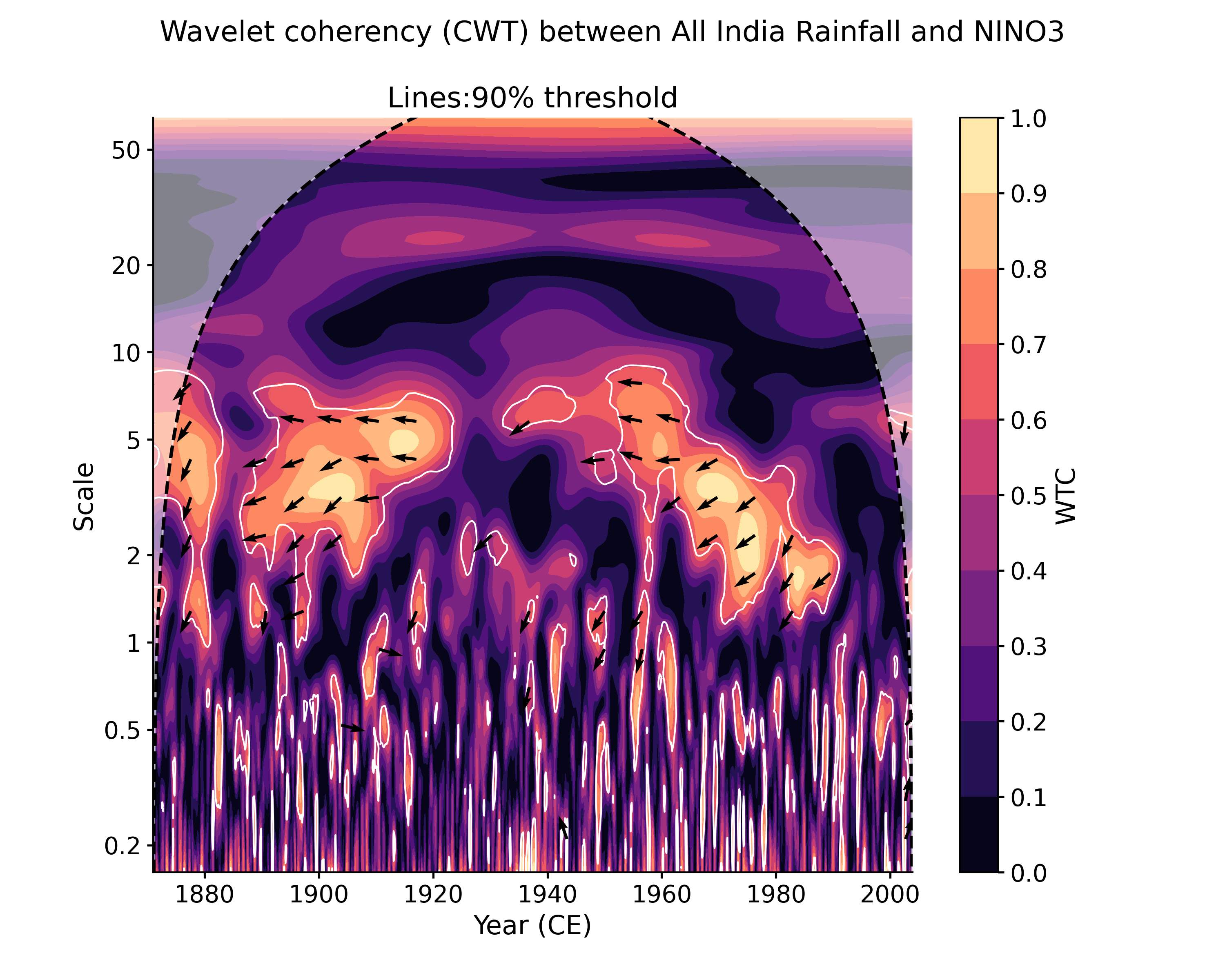
In [13]: cwt_sig = coh.signif_test(number=20, qs=[.9,.95]) # specifiying 2 significance thresholds does not take any more time.

# by default, the plot function will look for the closest quantile to 0.95, but it is easy to adjust:
In [14]: cwt_sig.plot(signif_thresh = 0.9)
Out[14]: 
(<Figure size 1000x800 with 2 Axes>,
 <AxesSubplot: title={'center': 'Lines:90% threshold'}, xlabel='Year (CE)', ylabel='Scale'>)

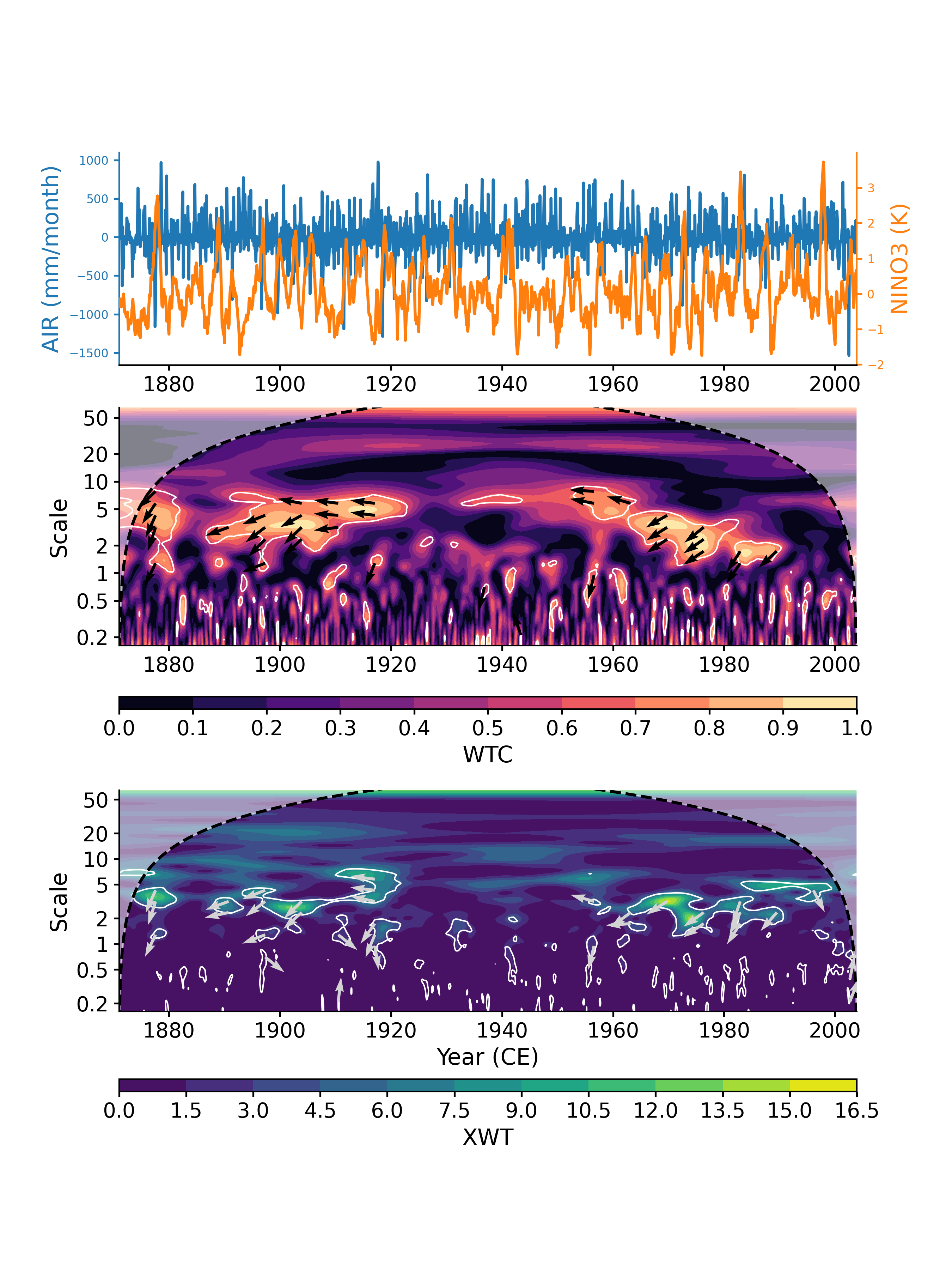
Another plotting option, dashboard, allows to visualize both timeseries as well as the wavelet transform coherency (WTC), which quantifies where two timeseries exhibit similar behavior in time-frequency space, and the cross-wavelet transform (XWT), which indicates regions of high common power.

In [15]: cwt_sig.dashboard()
Out[15]: 
(<Figure size 900x1200 with 6 Axes>,
 {'ts1': <AxesSubplot: ylabel='AIR (mm/month)'>,
  'ts2': <AxesSubplot: xlabel='Year (CE)', ylabel='NINO3 (K)'>,
  'wtc': <AxesSubplot: ylabel='Scale'>,
  'xwt': <AxesSubplot: xlabel='Year (CE)', ylabel='Scale'>})

Note: this design balances many considerations, and is not easily customizable.

MultipleSeries (pyleoclim.MultipleSeries)

class pyleoclim.core.multipleseries.MultipleSeries(series_list, time_unit=None, name=None)[source]

MultipleSeries object.

This object handles a collection of the type Series and can be created from a list of such objects. MultipleSeries should be used when the need to run analysis on multiple records arises, such as running principal component analysis. Some of the methods automatically transform the time axis prior to analysis to ensure consistency.

Parameters:

series_list (list) – a list of pyleoclim.Series objects
time_unit (str) – The target time unit for every series in the list. If None, then no conversion will be applied; Otherwise, the time unit of every series in the list will be converted to the target.
name (str) – name of the collection of timeseries (e.g. ‘PAGES 2k ice cores’)

Examples

In [1]: import pyleoclim as pyleo

In [2]: import pandas as pd

In [3]: data = pd.read_csv(
   ...:     'https://raw.githubusercontent.com/LinkedEarth/Pyleoclim_util/Development/example_data/soi_data.csv',
   ...:     skiprows=0, header=1
   ...: )
   ...: 

In [4]: time = data.iloc[:,1]

In [5]: value = data.iloc[:,2]

In [6]: ts1 = pyleo.Series(time=time, value=value, time_unit='years')

In [7]: ts2 = pyleo.Series(time=time, value=value, time_unit='years')

In [8]: ms = pyleo.MultipleSeries([ts1, ts2], name = 'SOI x2')

Methods

`append`(ts)	Append timeseries ts to MultipleSeries object
`bin`(**kwargs)	Aligns the time axes of a MultipleSeries object, via binning.
`common_time`([method, step, start, stop, ...])	Aligns the time axes of a MultipleSeries object
`convert_time_unit`([time_unit])	Convert the time units of the object
`copy`()	Copy the object
`correlation`([target, timespan, alpha, ...])	Calculate the correlation between a MultipleSeries and a target Series
`detrend`([method])	Detrend timeseries
`equal_lengths`()	Test whether all series in object have equal length
`filter`([cutoff_freq, cutoff_scale, method])	Filtering the timeseries in the MultipleSeries object
`flip`([axis])	Flips the Series along one or both axes
`gkernel`(**kwargs)	Aligns the time axes of a MultipleSeries object, via Gaussian kernel.
`increments`([step_style, verbose])	Extract grid properties (start, stop, step) of all the Series objects in a collection.
`interp`(**kwargs)	Aligns the time axes of a MultipleSeries object, via interpolation.
`pca`([weights, missing, tol_em, max_em_iter])	Principal Component Analysis (Empirical Orthogonal Functions)
`plot`([figsize, marker, markersize, ...])	Plot multiple timeseries on the same axis
`spectral`([method, settings, mute_pbar, ...])	Perform spectral analysis on the timeseries
`stackplot`([figsize, savefig_settings, xlim, ...])	Stack plot of multiple series
`standardize`()	Standardize each series object in a collection
`stripes`([ref_period, figsize, ...])	Represents a MultipleSeries object as a quilt of Ed Hawkins' "stripes" patterns
`wavelet`([method, settings, freq_method, ...])	Wavelet analysis

append(ts)[source]

Append timeseries ts to MultipleSeries object

Parameters:: ts (pyleoclim.Series) – The pyleoclim Series object to be appended to the MultipleSeries object
Returns:: ms – The augmented object, comprising the old one plus ts
Return type:: MultipleSeries

See also

pyleoclim.core.series.Series: A Pyleoclim Series object

Examples

In [1]: import pyleoclim as pyleo

In [2]: import pandas as pd

In [3]: data = pd.read_csv(
   ...:     'https://raw.githubusercontent.com/LinkedEarth/Pyleoclim_util/Development/example_data/soi_data.csv',
   ...:     skiprows=0, header=1
   ...: )
   ...: 

In [4]: time = data.iloc[:,1]

In [5]: value = data.iloc[:,2]

In [6]: ts1 = pyleo.Series(time=time, value=value, time_unit='years')

In [7]: ts2 = pyleo.Series(time=time, value=value, time_unit='years')

In [8]: ms = pyleo.MultipleSeries([ts1], name = 'SOI x2')

In [9]: ms.append(ts2)
Out[9]: <pyleoclim.core.multipleseries.MultipleSeries at 0x7f17f51420e0>

bin(**kwargs)[source]

Aligns the time axes of a MultipleSeries object, via binning.

This is critical for workflows that need to assume a common time axis for the group of series under consideration.

The common time axis is characterized by the following parameters:

start : the latest start date of the bunch (maximin of the minima)

stop : the earliest stop date of the bunch (minimum of the maxima)

step : The representative spacing between consecutive values (mean of the median spacings)

This is a special case of the common_time function.

Parameters:: kwargs (dict) – Arguments for the binning function. See pyleoclim.utils.tsutils.bin
Returns:: ms – The MultipleSeries objects with all series aligned to the same time axis.
Return type:: MultipleSeries

See also

pyleoclim.core.multipleseries.MultipleSeries.common_time: Base function on which this operates
pyleoclim.utils.tsutils.bin: Underlying binning function
pyleoclim.core.series.Series.bin: Bin function for Series object

Examples

In [1]: import pyleoclim as pyleo

In [2]: url = 'http://wiki.linked.earth/wiki/index.php/Special:WTLiPD?op=export&lipdid=MD982176.Stott.2004'

In [3]: data = pyleo.Lipd(usr_path = url)
Disclaimer: LiPD files may be updated and modified to adhere to standards

reading: MD982176.Stott.2004.lpd
Finished read: 1 record

In [4]: tslist = data.to_LipdSeriesList()
extracting paleoData...
extracting: MD982176.Stott.2004
Created time series: 6 entries

In [5]: tslist = tslist[2:] # drop the first two series which only concerns age and depth

In [6]: ms = pyleo.MultipleSeries(tslist)

In [7]: msbin = ms.bin()

common_time(method='interp', step=None, start=None, stop=None, step_style=None, **kwargs)[source]

Aligns the time axes of a MultipleSeries object

The alignment is achieved via binning, interpolation, or Gaussian kernel. Alignment is critical for workflows that need to assume a common time axis for the group of series under consideration.

The common time axis is characterized by the following parameters:

start : the latest start date of the bunch (maximun of the minima)

stop : the earliest stop date of the bunch (minimum of the maxima)

step : The representative spacing between consecutive values

Optional arguments for binning, Gaussian kernel (gkernel) interpolation are those of the underling functions.

If any of the time axes are retrograde, this step makes them prograde.

Parameters:

method (string; {'bin','interp','gkernel'}) – either ‘bin’, ‘interp’ [default] or ‘gkernel’
step (float) – common step for all time axes. Default is None and inferred from the timeseries spacing
start (float) – starting point of the common time axis. Default is None and inferred as the max of the min of the time axes for the timeseries.
stop (float) – end point of the common time axis. Default is None and inferred as the min of the max of the time axes for the timeseries.
step_style (string; {'median', 'mean', 'mode', 'max'}) – Method to obtain a representative step among all Series (using tsutils.increments). Default value is None, so that it will be chosen according to the method: ‘max’ for bin and gkernel, ‘mean’ for interp.
kwargs (dict) – keyword arguments (dictionary) of the bin, gkernel or interp methods

Returns:

ms – The MultipleSeries objects with all series aligned to the same time axis.

Return type:

MultipleSeries

See also

pyleoclim.utils.tsutils.bin: put timeseries values into bins of equal size (possibly leaving NaNs in).
pyleoclim.utils.tsutils.gkernel: coarse-graining using a Gaussian kernel
pyleoclim.utils.tsutils.interp: interpolation onto a regular grid (default = linear interpolation)
pyleoclim.utils.tsutils.increments: infer grid properties

Examples

In [1]: import numpy as np

In [2]: import pyleoclim as pyleo

In [3]: import matplotlib.pyplot as plt

In [4]: from pyleoclim.utils.tsmodel import colored_noise

# create 2 incompletely sampled series
In [5]: ns = 2 ; nt = 200; n_del = 20

In [6]: serieslist = []

In [7]: for j in range(ns):
   ...:     t = np.arange(nt)
   ...:     v = colored_noise(alpha=1, t=t)
   ...:     deleted_idx = np.random.choice(range(np.size(t)), n_del, replace=False)
   ...:     tu =  np.delete(t, deleted_idx)
   ...:     vu =  np.delete(v, deleted_idx)
   ...:     ts = pyleo.Series(time = tu, value = vu, label = 'series ' + str(j+1))
   ...:     serieslist.append(ts)
   ...: 

# create MS object from the list
In [8]: ms = pyleo.MultipleSeries(serieslist)

In [9]: fig, ax = plt.subplots(2,2,sharex=True,sharey=True, figsize=(10,8))

In [10]: ax = ax.flatten()

# apply common_time with default parameters
In [11]: msc = ms.common_time()

In [12]: msc.plot(title='linear interpolation',ax=ax[0], legend=False)
Out[12]: <AxesSubplot: title={'center': 'linear interpolation'}, xlabel='time', ylabel='value'>

# apply common_time with binning
In [13]: msc = ms.common_time(method='bin')

In [14]: msc.plot(title='Binning',ax=ax[1], legend=False)
Out[14]: <AxesSubplot: title={'center': 'Binning'}, xlabel='time', ylabel='value'>

# apply common_time with gkernel
In [15]: msc = ms.common_time(method='gkernel')

In [16]: msc.plot(title=r'Gaussian kernel ($h=3$)',ax=ax[2],legend=False)
Out[16]: <AxesSubplot: title={'center': 'Gaussian kernel ($h=3$)'}, xlabel='time', ylabel='value'>

# apply common_time with gkernel and a large bandwidth
In [17]: msc = ms.common_time(method='gkernel', h=.5)

In [18]: msc.plot(title=r'Gaussian kernel ($h=.5$)',ax=ax[3],legend=False)
Out[18]: <AxesSubplot: title={'center': 'Gaussian kernel ($h=.5$)'}, xlabel='time', ylabel='value'>

In [19]: fig.tight_layout()

# Optional close fig after plotting
In [20]: pyleo.closefig(fig)

convert_time_unit(time_unit='years')[source]

Convert the time units of the object

Parameters:

time_unit (str) –

the target time unit, possible input: {

’year’, ‘years’, ‘yr’, ‘yrs’, ‘y BP’, ‘yr BP’, ‘yrs BP’, ‘year BP’, ‘years BP’, ‘ky BP’, ‘kyr BP’, ‘kyrs BP’, ‘ka BP’, ‘ka’, ‘my BP’, ‘myr BP’, ‘myrs BP’, ‘ma BP’, ‘ma’,

}

Examples

In [1]: import pyleoclim as pyleo

In [2]: import pandas as pd

In [3]: data = pd.read_csv(
   ...:     'https://raw.githubusercontent.com/LinkedEarth/Pyleoclim_util/Development/example_data/soi_data.csv',
   ...:     skiprows=0, header=1
   ...: )
   ...: 

In [4]: time = data.iloc[:,1]

In [5]: value = data.iloc[:,2]

In [6]: ts1 = pyleo.Series(time=time, value=value, time_unit='years')

In [7]: ts2 = pyleo.Series(time=time, value=value, time_unit='years')

In [8]: ms = pyleo.MultipleSeries([ts1, ts2])

In [9]: new_ms = ms.convert_time_unit('yr BP')

In [10]: print('Original timeseries:')
Original timeseries:

In [11]: print('time unit:', ms.time_unit)
time unit: None

In [12]: print()


In [13]: print('Converted timeseries:')
Converted timeseries:

In [14]: print('time unit:', new_ms.time_unit)
time unit: yr BP

copy()[source]

Copy the object

Returns:: ms – The copied version of the pyleoclim.MultipleSeries object
Return type:: MultipleSeries

Examples

In [1]: import pyleoclim as pyleo

In [2]: import pandas as pd

In [3]: data = pd.read_csv(
   ...:     'https://raw.githubusercontent.com/LinkedEarth/Pyleoclim_util/Development/example_data/soi_data.csv',
   ...:     skiprows=0, header=1
   ...: )
   ...: 

In [4]: time = data.iloc[:,1]

In [5]: value = data.iloc[:,2]

In [6]: ts1 = pyleo.Series(time=time, value=value, time_unit='years')

In [7]: ts2 = pyleo.Series(time=time, value=value, time_unit='years')

In [8]: ms = pyleo.MultipleSeries([ts1], name = 'SOI x2')

In [9]: ms_copy = ms.copy()

correlation(target=None, timespan=None, alpha=0.05, settings=None, fdr_kwargs=None, common_time_kwargs=None, mute_pbar=False, seed=None)[source]

Calculate the correlation between a MultipleSeries and a target Series

Parameters:

target (pyleoclim.Series, optional) – The Series against which to take the correlation. If the target Series is not specified, then the 1st member of MultipleSeries will be used as the target
timespan (tuple, optional) – The time interval over which to perform the calculation
alpha (float) – The significance level (0.05 by default)
settings (dict) –
Parameters for the correlation function, including:

nsimint
the number of simulations (default: 1000)

methodstr, {‘ttest’,’isopersistent’,’isospectral’ (default)}
method for significance testing
fdr_kwargs (dict) – Parameters for the FDR function
common_time_kwargs (dict) – Parameters for the method MultipleSeries.common_time()
mute_pbar (bool; {True,False}) – If True, the progressbar will be muted. Default is False.
seed (float or int) – random seed for isopersistent and isospectral methods

Returns:

corr – the result object

Return type:

CorrEns

See also

pyleoclim.utils.correlation.corr_sig: Correlation function
pyleoclim.utils.correlation.fdr: FDR function
pyleoclim.core.correns.CorrEns: the correlation ensemble object

Examples

In [1]: import pyleoclim as pyleo

In [2]: from pyleoclim.utils.tsmodel import colored_noise

In [3]: import numpy as np

In [4]: nt = 100

In [5]: t0 = np.arange(nt)

In [6]: v0 = colored_noise(alpha=1, t=t0)

In [7]: noise = np.random.normal(loc=0, scale=1, size=nt)

In [8]: ts0 = pyleo.Series(time=t0, value=v0)

In [9]: ts1 = pyleo.Series(time=t0, value=v0+noise)

In [10]: ts2 = pyleo.Series(time=t0, value=v0+2*noise)

In [11]: ts3 = pyleo.Series(time=t0, value=v0+1/2*noise)

In [12]: ts_list = [ts1, ts2, ts3]

In [13]: ms = pyleo.MultipleSeries(ts_list)

In [14]: ts_target = ts0

Correlation between the MultipleSeries object and a target Series. We also set an arbitrary random seed to ensure reproducibility:

In [15]: corr_res = ms.correlation(ts_target, settings={'nsim': 20}, seed=2333)
Looping over 3 Series in collection

In [16]: print(corr_res)
  correlation  p-value    signif. w/o FDR (α: 0.05)    signif. w/ FDR (α: 0.05)
-------------  ---------  ---------------------------  --------------------------
     0.997758  < 1e-6     True                         True
     0.991055  < 1e-6     True                         True
     0.99944   < 1e-6     True                         True
Ensemble size: 3

Correlation among the series of the MultipleSeries object

In [17]: corr_res = ms.correlation(settings={'nsim': 20}, seed=2333)
Looping over 3 Series in collection

In [18]: print(corr_res)
  correlation  p-value    signif. w/o FDR (α: 0.05)    signif. w/ FDR (α: 0.05)
-------------  ---------  ---------------------------  --------------------------
     1         < 1e-6     True                         True
     0.997764  < 1e-6     True                         True
     0.999439  < 1e-6     True                         True
Ensemble size: 3

detrend(method='emd', **kwargs)[source]

Detrend timeseries

Parameters:

method (str, optional) –
The method for detrending. The default is ‘emd’. Options include:
- linear: the result of a linear least-squares fit to y is subtracted from y.
- constant: only the mean of data is subtrated.
- ’savitzky-golay’, y is filtered using the Savitzky-Golay filters and the resulting filtered series is subtracted from y.
- ’emd’ (default): Empirical mode decomposition. The last mode is assumed to be the trend and removed from the series
**kwargs (dict) – Relevant arguments for each of the methods.

Returns:

ms – The detrended timeseries

Return type:

MultipleSeries

See also

pyleoclim.core.series.Series.detrend: Detrending for a single series
pyleoclim.utils.tsutils.detrend: Detrending function

equal_lengths()[source]

Test whether all series in object have equal length

Returns:

flag (bool) – Whether or not the Series in the pyleo.MultipleSeries object are of equal length
lengths (list) – List of the lengths of the series in object

See also

pyleoclim.core.multipleseries.MultipleSeries.common_time: Aligns the time axes of a MultipleSeries object

Examples

In [1]: import pyleoclim as pyleo

In [2]: import pandas as pd

In [3]: data = pd.read_csv(
   ...:     'https://raw.githubusercontent.com/LinkedEarth/Pyleoclim_util/Development/example_data/soi_data.csv',
   ...:     skiprows=0, header=1
   ...: )
   ...: 

In [4]: time = data.iloc[:,1]

In [5]: value = data.iloc[:,2]

In [6]: ts1 = pyleo.Series(time=time, value=value, time_unit='years')

In [7]: ts2 = pyleo.Series(time=time, value=value, time_unit='years')

In [8]: ms = pyleo.MultipleSeries([ts1], name = 'SOI x2')

In [9]: flag, lengths = ms.equal_lengths()

In [10]: print(flag)
True

filter(cutoff_freq=None, cutoff_scale=None, method='butterworth', **kwargs)[source]

Filtering the timeseries in the MultipleSeries object

Parameters:

method (str; {'savitzky-golay', 'butterworth', 'firwin', 'lanczos'}) – The filtering method - ‘butterworth’: the Butterworth method (default) - ‘savitzky-golay’: the Savitzky-Golay method - ‘firwin’: FIR filter design using the window method, with default window as Hamming - ‘lanczos’: lowpass filter via Lanczos resampling
cutoff_freq (float or list) – The cutoff frequency only works with the Butterworth method. If a float, it is interpreted as a low-frequency cutoff (lowpass). If a list, it is interpreted as a frequency band (f1, f2), with f1 < f2 (bandpass).
cutoff_scale (float or list) – cutoff_freq = 1 / cutoff_scale The cutoff scale only works with the Butterworth method and when cutoff_freq is None. If a float, it is interpreted as a low-frequency (high-scale) cutoff (lowpass). If a list, it is interpreted as a frequency band (f1, f2), with f1 < f2 (bandpass).
kwargs (dict) – A dictionary of the keyword arguments for the filtering method, See pyleoclim.utils.filter.savitzky_golay, pyleoclim.utils.filter.butterworth, pyleoclim.utils.filter.firwin, and pyleoclim.utils.filter.lanczos for the details

Returns:

ms

Return type:

MultipleSeries

See also

pyleoclim.series.Series.filter: filtering for Series objects
pyleoclim.utils.filter.butterworth: Butterworth method
pyleoclim.utils.filter.savitzky_golay: Savitzky-Golay method
pyleoclim.utils.filter.firwin: FIR filter design using the window method
pyleoclim.utils.filter.lanczos: lowpass filter via Lanczos resampling

Examples

In [1]: import pyleoclim as pyleo

In [2]: import pandas as pd

In [3]: data = pd.read_csv(
   ...:     'https://raw.githubusercontent.com/LinkedEarth/Pyleoclim_util/Development/example_data/soi_data.csv',
   ...:     skiprows=0, header=1
   ...: )
   ...: 

In [4]: time = data.iloc[:,1]

In [5]: value = data.iloc[:,2]

In [6]: ts1 = pyleo.Series(time=time, value=value, time_unit='years')

In [7]: ts2 = pyleo.Series(time=time, value=value, time_unit='years')

In [8]: ms = pyleo.MultipleSeries([ts1, ts2], name = 'SOI x2')

In [9]: ms_filter = ms.filter(method='lanczos',cutoff_scale=20)

flip(axis='value')[source]

Flips the Series along one or both axes

Parameters:

axis (str, optional) – The axis along which the Series will be flipped. The default is ‘value’. Other acceptable options are ‘time’ or ‘both’. TODO: enable time flipping after paleopandas is released

Returns:

ms – The flipped object

Examples

In [1]: import pyleoclim as pyleo

In [2]: url = 'http://wiki.linked.earth/wiki/index.php/Special:WTLiPD?op=export&lipdid=MD982176.Stott.2004'

In [3]: data = pyleo.Lipd(usr_path = url)
Disclaimer: LiPD files may be updated and modified to adhere to standards

reading: MD982176.Stott.2004.lpd
Finished read: 1 record

In [4]: tslist = data.to_LipdSeriesList()
extracting paleoData...
extracting: MD982176.Stott.2004
Created time series: 6 entries

In [5]: tslist = tslist[2:] # drop the first two series which only concerns age and depth

In [6]: ms = pyleo.MultipleSeries(tslist)

In [7]: fig, ax = ms.flip().stackplot()

In [8]: pyleo.closefig(fig)

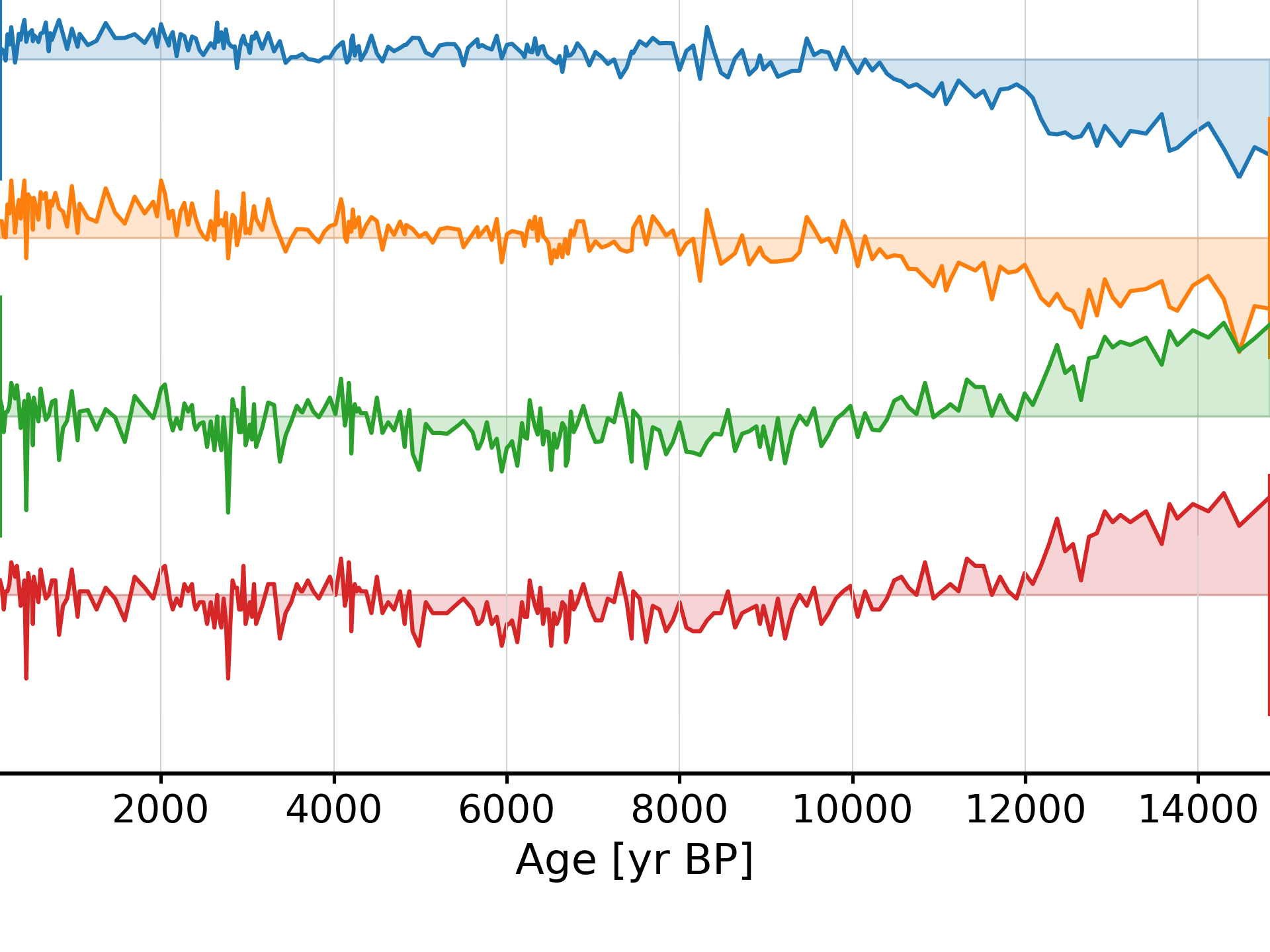
Return type:

MultipleSeries

Note that labels have been updated to reflect the flip

gkernel(**kwargs)[source]

Aligns the time axes of a MultipleSeries object, via Gaussian kernel.

This is critical for workflows that need to assume a common time axis for the group of series under consideration.

The common time axis is characterized by the following parameters:

start : the latest start date of the bunch (maximin of the minima)

stop : the earliest stop date of the bunch (minimum of the maxima)

step : The representative spacing between consecutive values (mean of the median spacings)

This is a special case of the common_time function.

Parameters:: kwargs (dict) – Arguments for gkernel. See pyleoclim.utils.tsutils.gkernel for details.
Returns:: ms – The MultipleSeries objects with all series aligned to the same time axis.
Return type:: MultipleSeries

See also

pyleoclim.core.multipleseries.MultipleSeries.common_time: Base function on which this operates
pyleoclim.utils.tsutils.gkernel: Underlying kernel module

Examples

In [1]: import pyleoclim as pyleo

In [2]: url = 'http://wiki.linked.earth/wiki/index.php/Special:WTLiPD?op=export&lipdid=MD982176.Stott.2004'

In [3]: data = pyleo.Lipd(usr_path = url)
Disclaimer: LiPD files may be updated and modified to adhere to standards

reading: MD982176.Stott.2004.lpd
Finished read: 1 record

In [4]: tslist = data.to_LipdSeriesList()
extracting paleoData...
extracting: MD982176.Stott.2004
Created time series: 6 entries

In [5]: tslist = tslist[2:] # drop the first two series which only concerns age and depth

In [6]: ms = pyleo.MultipleSeries(tslist)

In [7]: msk = ms.gkernel()

increments(step_style='median', verbose=False)[source]

Extract grid properties (start, stop, step) of all the Series objects in a collection.

Parameters:

step_style (str; {'median','mean','mode','max'}) –
Method to obtain a representative step if x is not evenly spaced. Valid entries: ‘median’ [default], ‘mean’, ‘mode’ or ‘max’. The “mode” is the most frequent entry in a dataset, and may be a good choice if the timeseries is nearly equally spaced but for a few gaps.

”max” is a conservative choice, appropriate for binning methods and Gaussian kernel coarse-graining
verbose (bool) – If True, will print out warning messages when they appear

Returns:

increments – n x 3 array, where n is the number of series,

index 0 is the earliest time among all Series
index 1 is the latest time among all Series
index 2 is the step, chosen according to step_style

Return type:

numpy.array

See also

pyleoclim.utils.tsutils.increments: underlying array-level utility

Examples

In [1]: import pyleoclim as pyleo

In [2]: import pandas as pd

In [3]: data = pd.read_csv(
   ...:     'https://raw.githubusercontent.com/LinkedEarth/Pyleoclim_util/Development/example_data/soi_data.csv',
   ...:     skiprows=0, header=1
   ...: )
   ...: 

In [4]: time = data.iloc[:,1]

In [5]: value = data.iloc[:,2]

In [6]: ts1 = pyleo.Series(time=time, value=value, time_unit='years')

In [7]: ts2 = pyleo.Series(time=time, value=value, time_unit='years')

In [8]: ms = pyleo.MultipleSeries([ts1], name = 'SOI x2')

In [9]: increments = ms.increments()

interp(**kwargs)[source]

Aligns the time axes of a MultipleSeries object, via interpolation.

This is critical for workflows that need to assume a common time axis for the group of series under consideration.

The common time axis is characterized by the following parameters:

start : the latest start date of the bunch (maximin of the minima)

stop : the earliest stop date of the bunch (minimum of the maxima)

step : The representative spacing between consecutive values (mean of the median spacings)

This is a special case of the common_time function.

Parameters:: kwargs (keyword arguments (dictionary) for the interpolation method) –
Returns:: ms – The MultipleSeries objects with all series aligned to the same time axis.
Return type:: MultipleSeries

See also

pyleoclim.core.multipleseries.MultipleSeries.common_time: Base function on which this operates
pyleoclim.utils.tsutils.interp: Underlying interpolation function
pyleoclim.core.series.Series.interp: Interpolation function for Series object

Examples

In [1]: import pyleoclim as pyleo

In [2]: url = 'http://wiki.linked.earth/wiki/index.php/Special:WTLiPD?op=export&lipdid=MD982176.Stott.2004'

In [3]: data = pyleo.Lipd(usr_path = url)
Disclaimer: LiPD files may be updated and modified to adhere to standards

reading: MD982176.Stott.2004.lpd
Finished read: 1 record

In [4]: tslist = data.to_LipdSeriesList()
extracting paleoData...
extracting: MD982176.Stott.2004
Created time series: 6 entries

In [5]: tslist = tslist[2:] # drop the first two series which only concerns age and depth

In [6]: ms = pyleo.MultipleSeries(tslist)

In [7]: msinterp = ms.interp()

pca(weights=None, missing='fill-em', tol_em=0.005, max_em_iter=100, **pca_kwargs)[source]

Principal Component Analysis (Empirical Orthogonal Functions)

Decomposition of dataset ys in terms of orthogonal basis functions. Tolerant to missing values, infilled by an EM algorithm.

Do make sure the time axes are aligned, however! (e.g. use common_time())

Algorithm from statsmodels: https://www.statsmodels.org/stable/generated/statsmodels.multivariate.pca.PCA.html

Parameters:

weights (ndarray, optional) – Series weights to use after transforming data according to standardize or demean when computing the principal components.
missing ({str, None}) –
Method for missing data. Choices are:
- ’drop-row’ - drop rows with missing values.
- ’drop-col’ - drop columns with missing values.
- ’drop-min’ - drop either rows or columns, choosing by data retention.
- ’fill-em’ - use EM algorithm to fill missing value. ncomp should be set to the number of factors required.
- None raises if data contains NaN values.
tol_em (float) – Tolerance to use when checking for convergence of the EM algorithm.
max_em_iter (int) – Maximum iterations for the EM algorithm.

Returns:

res – Resulting pyleoclim.SpatialDecomp object

Return type:

SpatialDecomp

See also

pyleoclim.utils.tsutils.eff_sample_size: Effective Sample Size of timeseries y
pyleoclim.core.spatialdecomp.SpatialDecomp: The spatial decomposition object

Examples

In [1]: import pyleoclim as pyleo

In [2]: url = 'http://wiki.linked.earth/wiki/index.php/Special:WTLiPD?op=export&lipdid=MD982176.Stott.2004'

In [3]: data = pyleo.Lipd(usr_path = url)
Disclaimer: LiPD files may be updated and modified to adhere to standards

reading: MD982176.Stott.2004.lpd
Finished read: 1 record

In [4]: tslist = data.to_LipdSeriesList()
extracting paleoData...
extracting: MD982176.Stott.2004
Created time series: 6 entries

In [5]: tslist = tslist[2:] # drop the first two series which only concerns age and depth

In [6]: ms = pyleo.MultipleSeries(tslist).common_time()

In [7]: res = ms.pca() # carry out PCA

In [8]: fig1, ax1 = res.screeplot() # plot the eigenvalue spectrum

In [9]: pyleo.closefig(fig1)    # Optional close fig after plotting

In [10]: fig2, ax2 = res.modeplot() # plot the first mode

In [11]: pyleo.closefig(fig2)    # Optional close fig after plotting

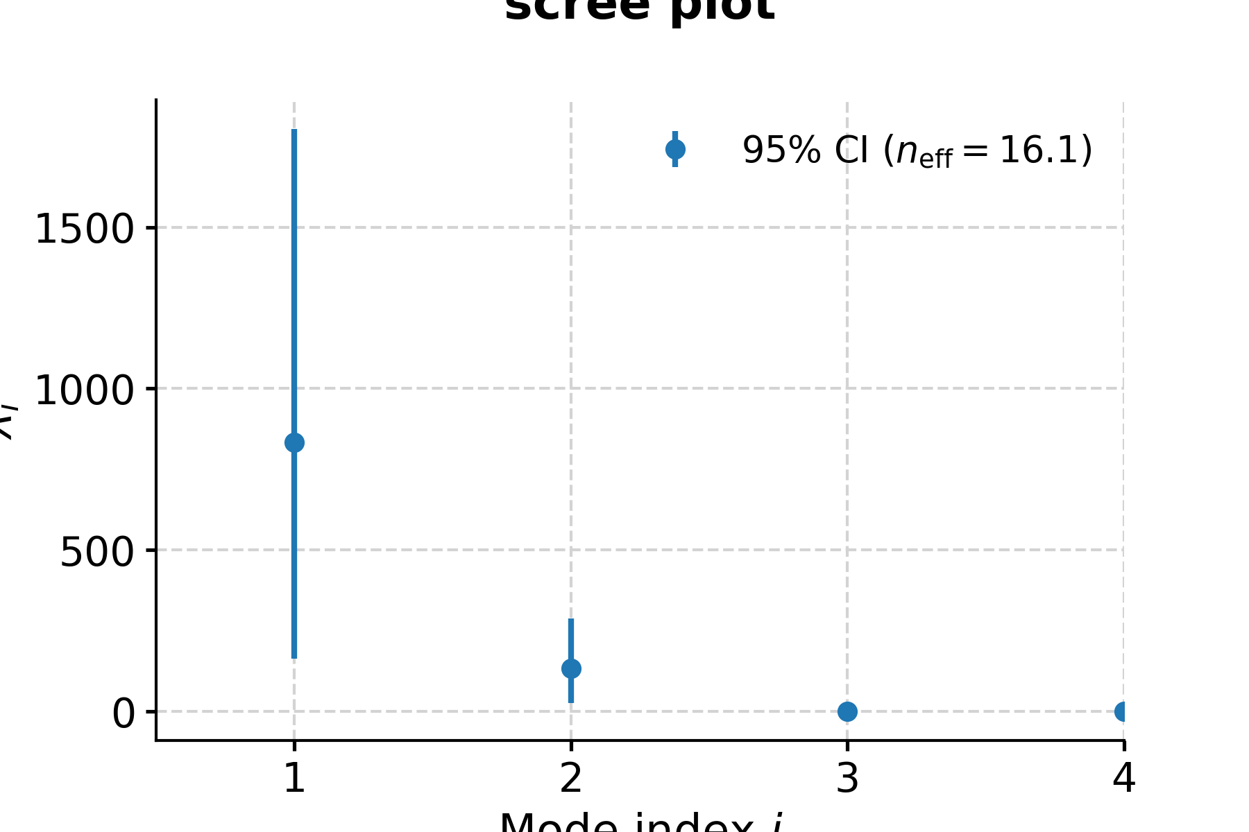
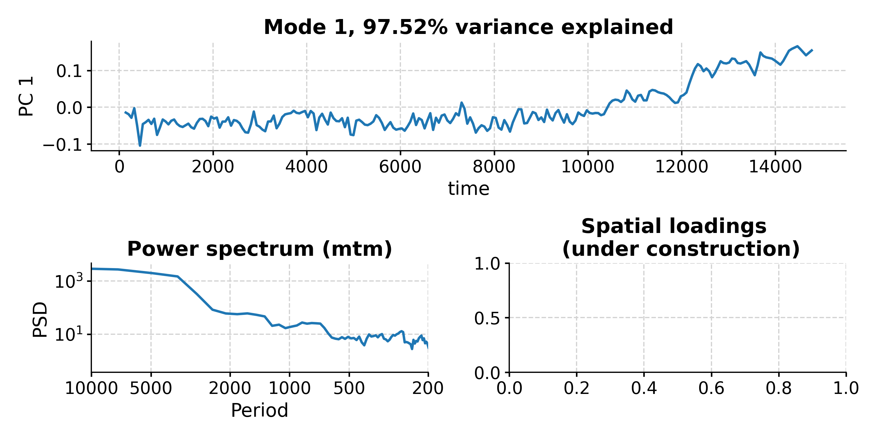
plot(figsize=[10, 4], marker=None, markersize=None, linestyle=None, linewidth=None, colors=None, cmap='tab10', norm=None, xlabel=None, ylabel=None, title=None, legend=True, plot_kwargs=None, lgd_kwargs=None, savefig_settings=None, ax=None, invert_xaxis=False)[source]

Plot multiple timeseries on the same axis

Parameters:

figsize (list, optional) – Size of the figure. The default is [10, 4].
marker (str, optional) – Marker type. The default is None.
markersize (float, optional) – Marker size. The default is None.
linestyle (str, optional) – Line style. The default is None.
linewidth (float, optional) – The width of the line. The default is None.
colors (a list of, or one, Python supported color code (a string of hex code or a tuple of rgba values)) – Colors for plotting. If None, the plotting will cycle the ‘tab10’ colormap; if only one color is specified, then all curves will be plotted with that single color; if a list of colors are specified, then the plotting will cycle that color list.
cmap (str) – The colormap to use when “colors” is None.
norm (matplotlib.colors.Normalize) – The normalization for the colormap. If None, a linear normalization will be used.
xlabel (str, optional) – x-axis label. The default is None.
ylabel (str, optional) – y-axis label. The default is None.
title (str, optional) – Title. The default is None.
legend (bool, optional) – Whether the show the legend. The default is True.
plot_kwargs (dict, optional) – Plot parameters. The default is None.
lgd_kwargs (dict, optional) – Legend parameters. The default is None.
savefig_settings (dictionary, optional) –
the dictionary of arguments for plt.savefig(); some notes below: - “path” must be specified; it can be any existing or non-existing path,

with or without a suffix; if the suffix is not given in “path”, it will follow “format”
- ”format” can be one of {“pdf”, “eps”, “png”, “ps”} The default is None.
ax (matplotlib.ax, optional) – The matplotlib axis onto which to return the figure. The default is None.
invert_xaxis (bool, optional) – if True, the x-axis of the plot will be inverted

Returns:

fig (matplotlib.figure) – the figure object from matplotlib See [matplotlib.pyplot.figure](https://matplotlib.org/3.1.1/api/_as_gen/matplotlib.pyplot.figure.html) for details.
ax (matplotlib.axis) – the axis object from matplotlib See [matplotlib.axes](https://matplotlib.org/api/axes_api.html) for details.

See also

pyleoclim.utils.plotting.savefig: Saving figure in Pyleoclim

Examples

In [1]: import pyleoclim as pyleo

In [2]: url = 'http://wiki.linked.earth/wiki/index.php/Special:WTLiPD?op=export&lipdid=MD982176.Stott.2004'

In [3]: data = pyleo.Lipd(usr_path = url)
Disclaimer: LiPD files may be updated and modified to adhere to standards

reading: MD982176.Stott.2004.lpd
Finished read: 1 record

In [4]: tslist = data.to_LipdSeriesList()
extracting paleoData...
extracting: MD982176.Stott.2004
Created time series: 6 entries

In [5]: tslist = tslist[2:] # drop the first two series which only concerns age and depth

In [6]: ms = pyleo.MultipleSeries(tslist)

In [7]: fig, ax = ms.plot()

In [8]: pyleo.closefig(fig) #Optional close fig after plotting

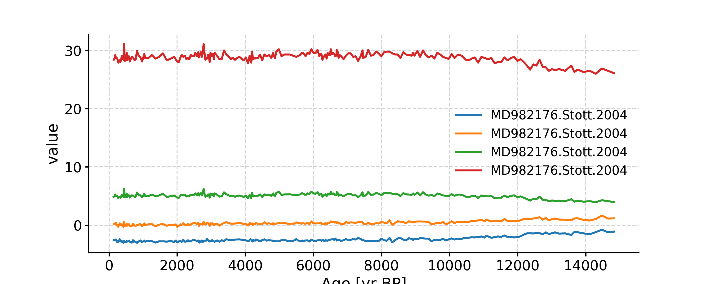
spectral(method='lomb_scargle', settings=None, mute_pbar=False, freq_method='log', freq_kwargs=None, label=None, verbose=False, scalogram_list=None)[source]

Perform spectral analysis on the timeseries

Parameters:

method (str; {'wwz', 'mtm', 'lomb_scargle', 'welch', 'periodogram', 'cwt'}) –
freq_method (str; {'log','scale', 'nfft', 'lomb_scargle', 'welch'}) –
freq_kwargs (dict) – Arguments for frequency vector
settings (dict) – Arguments for the specific spectral method
label (str) – Label for the PSD object
verbose (bool) – If True, will print warning messages if there is any
mute_pbar (bool) – Mute the progress bar. Default is False.
scalogram_list (pyleoclim.MultipleScalogram) – Multiple scalogram object containing pre-computed scalograms to use when calculating spectra, only works with wwz or cwt

Returns:

psd – A Multiple PSD object

Return type:

MultiplePSD

See also

pyleoclim.utils.spectral.mtm: Spectral analysis using the Multitaper approach
pyleoclim.utils.spectral.lomb_scargle: Spectral analysis using the Lomb-Scargle method
pyleoclim.utils.spectral.welch: Spectral analysis using the Welch segement approach
pyleoclim.utils.spectral.periodogram: Spectral anaysis using the basic Fourier transform
pyleoclim.utils.spectral.wwz_psd: Spectral analysis using the Wavelet Weighted Z transform
pyleoclim.utils.spectral.cwt_psd: Spectral analysis using the continuous Wavelet Transform as implemented by Torrence and Compo
pyleoclim.utils.wavelet.make_freq_vector: Functions to create the frequency vector
pyleoclim.utils.tsutils.detrend: Detrending function
pyleoclim.core.series.Series.spectral: Spectral analysis for a single timeseries
pyleoclim.core.PSD.PSD: PSD object
pyleoclim.core.psds.MultiplePSD: Multiple PSD object

Examples

In [1]: import pyleoclim as pyleo

In [2]: url = 'http://wiki.linked.earth/wiki/index.php/Special:WTLiPD?op=export&lipdid=MD982176.Stott.2004'

In [3]: data = pyleo.Lipd(usr_path = url)
Disclaimer: LiPD files may be updated and modified to adhere to standards

reading: MD982176.Stott.2004.lpd
Finished read: 1 record

In [4]: tslist = data.to_LipdSeriesList()
extracting paleoData...
extracting: MD982176.Stott.2004
Created time series: 6 entries

In [5]: tslist = tslist[2:] # drop the first two series which only concerns age and depth

In [6]: ms = pyleo.MultipleSeries(tslist)

In [7]: ms_psd = ms.spectral()

stackplot(figsize=None, savefig_settings=None, xlim=None, fill_between_alpha=0.2, colors=None, cmap='tab10', norm=None, labels='auto', spine_lw=1.5, grid_lw=0.5, label_x_loc=-0.15, v_shift_factor=0.75, linewidth=1.5, plot_kwargs=None)[source]

Stack plot of multiple series

Note that the plotting style is uniquely designed for this one and cannot be properly reset with pyleoclim.set_style().

Parameters:

figsize (list) – Size of the figure.
savefig_settings (dictionary) –
the dictionary of arguments for plt.savefig(); some notes below: - “path” must be specified; it can be any existing or non-existing path,

with or without a suffix; if the suffix is not given in “path”, it will follow “format”
- ”format” can be one of {“pdf”, “eps”, “png”, “ps”} The default is None.
xlim (list) – The x-axis limit.
fill_between_alpha (float) – The transparency for the fill_between shades.
colors (a list of, or one, Python supported color code (a string of hex code or a tuple of rgba values)) – Colors for plotting. If None, the plotting will cycle the ‘tab10’ colormap; if only one color is specified, then all curves will be plotted with that single color; if a list of colors are specified, then the plotting will cycle that color list.
cmap (str) – The colormap to use when “colors” is None.
norm (matplotlib.colors.Normalize like) – The nomorlization for the colormap. If None, a linear normalization will be used.
labels (None, 'auto' or list) – If None, doesn’t add labels to the subplots If ‘auto’, uses the labels passed during the creation of pyleoclim.Series If list, pass a list of strings for each labels. Default is ‘auto’
spine_lw (float) – The linewidth for the spines of the axes.
grid_lw (float) – The linewidth for the gridlines.
label_x_loc (float) – The x location for the label of each curve.
v_shift_factor (float) – The factor for the vertical shift of each axis. The default value 3/4 means the top of the next axis will be located at 3/4 of the height of the previous one.
linewidth (float) – The linewidth for the curves.
plot_kwargs (dict or list of dict) –
Arguments to further customize the plot from matplotlib.pyplot.plot.
- Dictionary: Arguments will be applied to all lines in the stackplots
- List of dictionary: Allows to customize one line at a time.

Returns:

fig (matplotlib.figure) – the figure object from matplotlib See [matplotlib.pyplot.figure](https://matplotlib.org/3.1.1/api/_as_gen/matplotlib.pyplot.figure.html) for details.
ax (matplotlib.axis) – the axis object from matplotlib See [matplotlib.axes](https://matplotlib.org/api/axes_api.html) for details.

See also

pyleoclim.utils.plotting.savefig: Saving figure in Pyleoclim

Examples

In [1]: import pyleoclim as pyleo

In [2]: url = 'http://wiki.linked.earth/wiki/index.php/Special:WTLiPD?op=export&lipdid=MD982176.Stott.2004'

In [3]: d = pyleo.Lipd(usr_path = url)
Disclaimer: LiPD files may be updated and modified to adhere to standards

reading: MD982176.Stott.2004.lpd
Finished read: 1 record

In [4]: tslist = d.to_LipdSeriesList()
extracting paleoData...
extracting: MD982176.Stott.2004
Created time series: 6 entries

In [5]: tslist = tslist[2:] # drop the first two series which only concerns age and depth

In [6]: ms = pyleo.MultipleSeries(tslist)

In [7]: fig, ax = ms.stackplot()

In [8]: pyleo.closefig(fig)

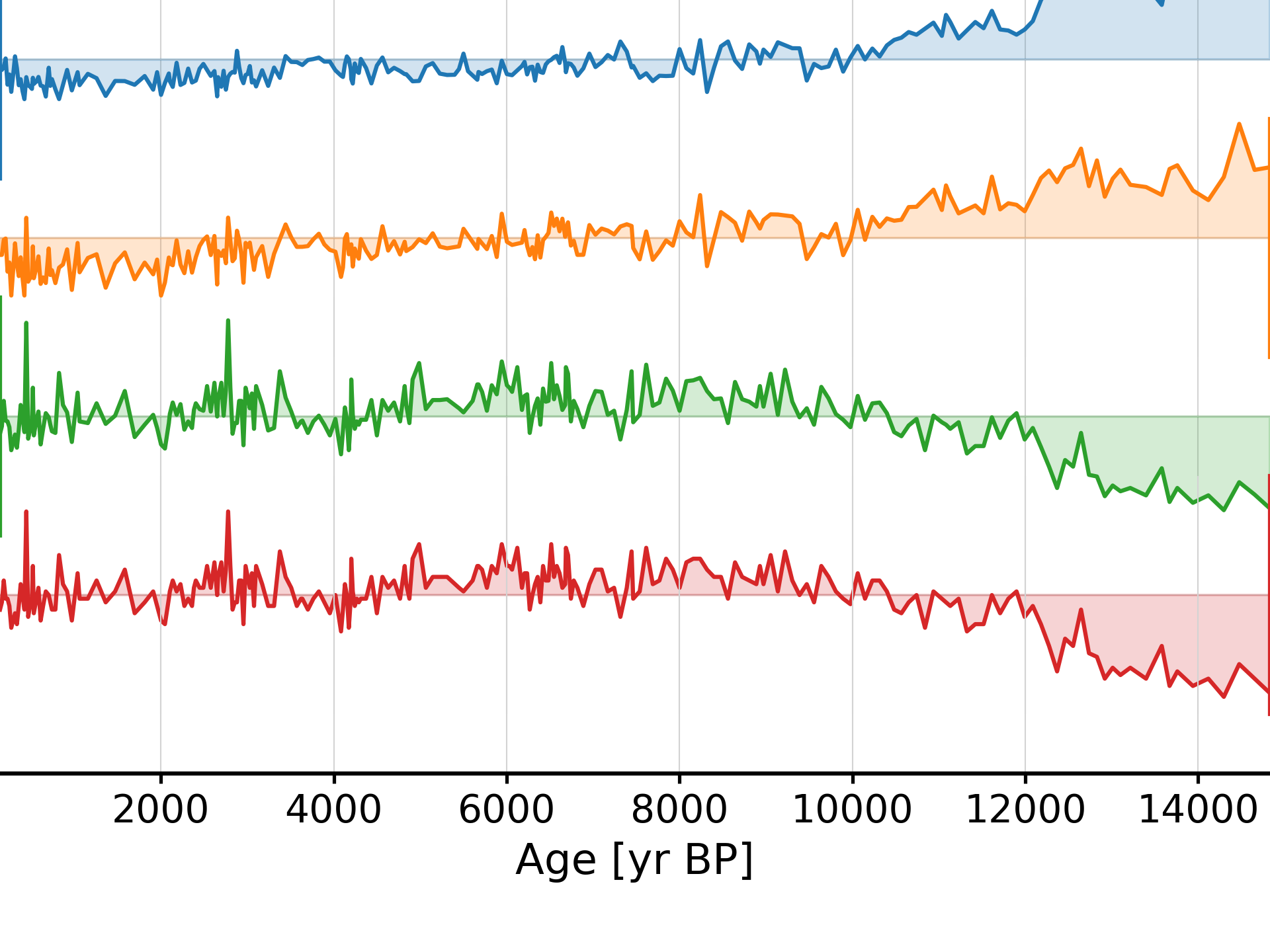
Let’s change the labels on the left

In [9]: sst = d.to_LipdSeries(number=5)
extracting paleoData...
extracting: MD982176.Stott.2004
Created time series: 6 entries

In [10]: d18Osw = d.to_LipdSeries(number=3)
extracting paleoData...
extracting: MD982176.Stott.2004
Created time series: 6 entries

In [11]: ms = pyleo.MultipleSeries([sst,d18Osw])

In [12]: fig, ax = ms.stackplot(labels=['sst','d18Osw'])

In [13]: pyleo.closefig(fig)

../_images/mts_stackplot_customlabels.png

And let’s remove them completely

In [14]: fig, ax = ms.stackplot(labels=None)

In [15]: pyleo.closefig(fig) #Optional figure close after plotting

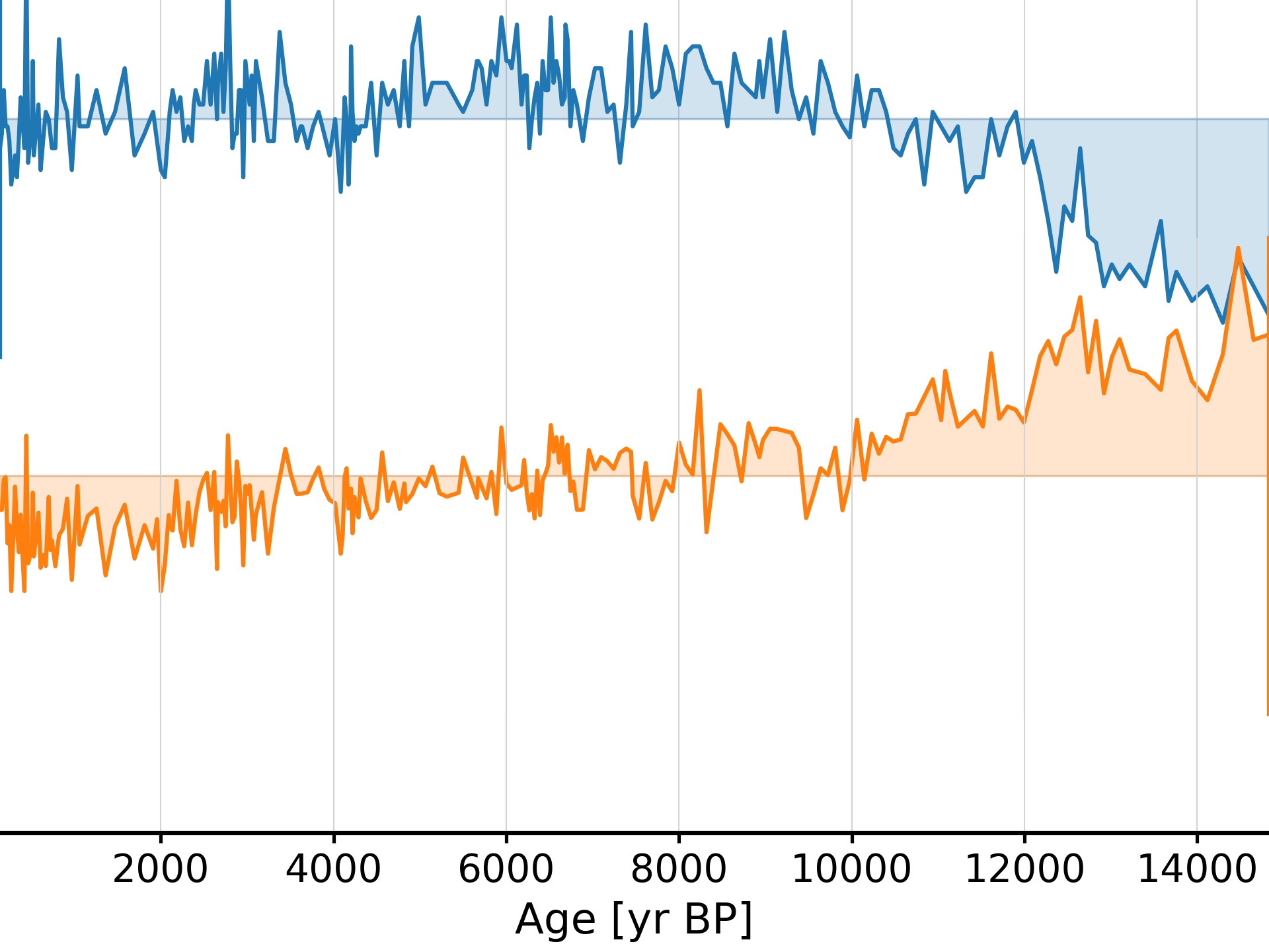
Now, let’s add markers to the timeseries.

In [16]: fig, ax = ms.stackplot(labels=None, plot_kwargs={'marker':'o'})

In [17]: pyleo.closefig(fig) #Optional figure close after plotting

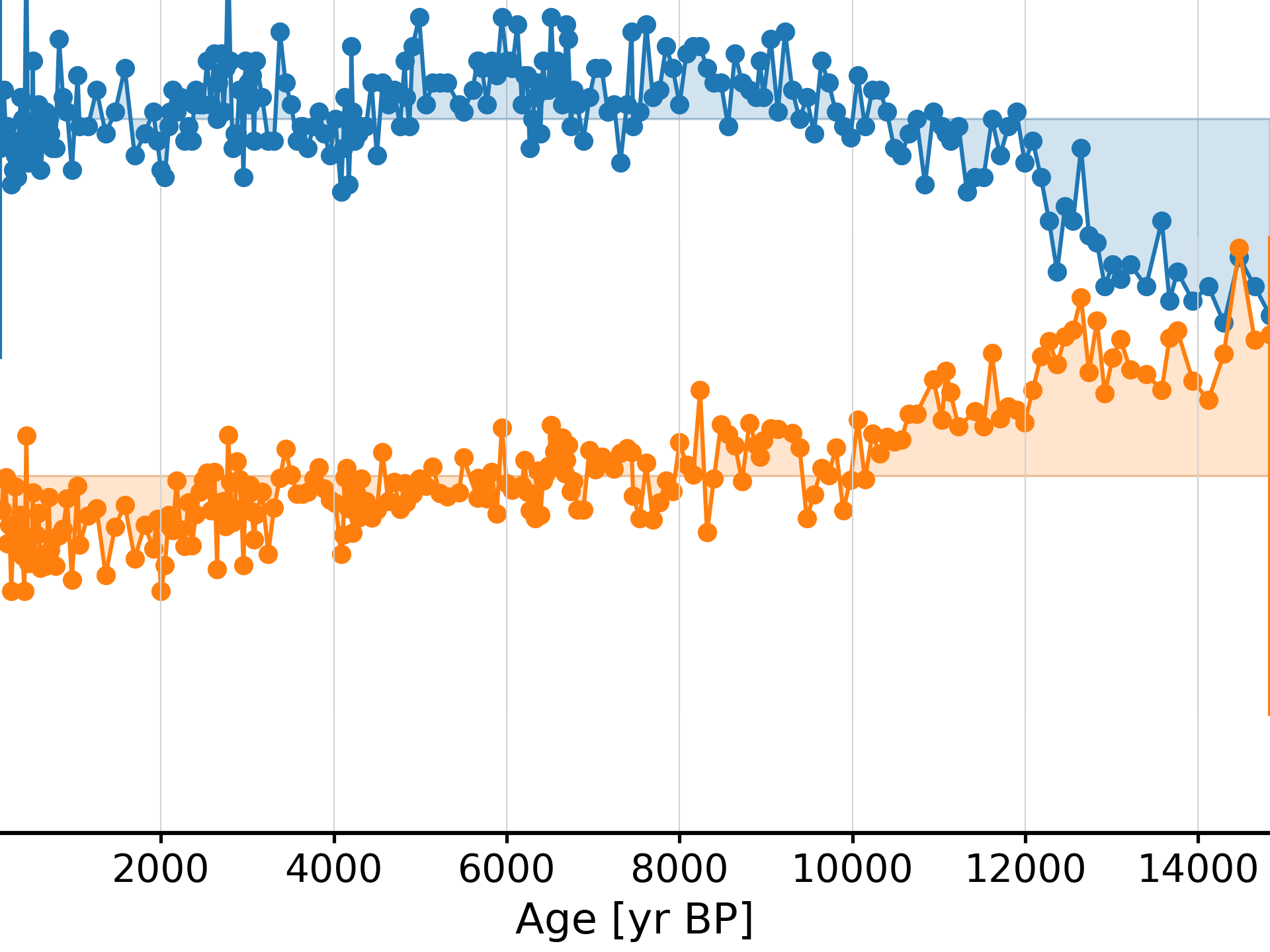
../_images/mts_stackplot_samemarkers.png

Using different marker types on each series:

In [18]: fig, ax = ms.stackplot(labels=None, plot_kwargs=[{'marker':'o'},{'marker':'^'}])

In [19]: pyleo.closefig(fig) #Optional figure close after plotting

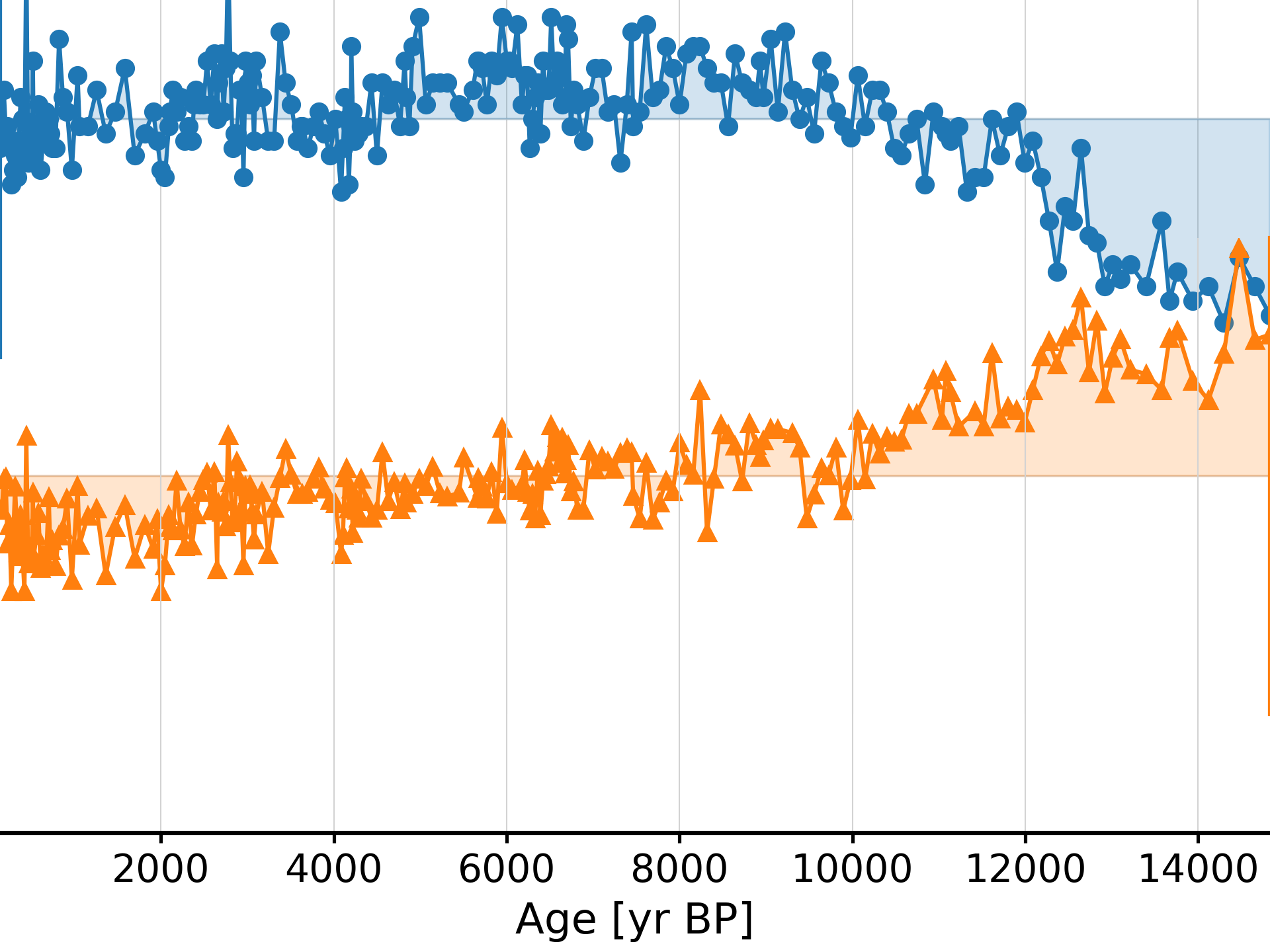
../_images/mts_stackplot_differentmarkers.png

standardize()[source]

Standardize each series object in a collection

Returns:: ms – The standardized pyleoclim.MultipleSeries object
Return type:: MultipleSeries

Examples

In [1]: import pyleoclim as pyleo

In [2]: import pandas as pd

In [3]: data = pd.read_csv(
   ...:     'https://raw.githubusercontent.com/LinkedEarth/Pyleoclim_util/Development/example_data/soi_data.csv',
   ...:     skiprows=0, header=1
   ...: )
   ...: 

In [4]: time = data.iloc[:,1]

In [5]: value = data.iloc[:,2]

In [6]: ts1 = pyleo.Series(time=time, value=value, time_unit='years')

In [7]: ts2 = pyleo.Series(time=time, value=value, time_unit='years')

In [8]: ms = pyleo.MultipleSeries([ts1], name = 'SOI x2')

In [9]: ms_std = ms.standardize()

stripes(ref_period=None, figsize=None, savefig_settings=None, LIM=2.8, thickness=1.0, labels='auto', label_color='gray', common_time_kwargs=None, xlim=None, font_scale=0.8, x_offset=0.05)[source]

Represents a MultipleSeries object as a quilt of Ed Hawkins’ “stripes” patterns

To ensure comparability, constituent series are placed on a common time axis, using MultipleSeries.common_time(). To ensure consistent scaling, all series are Gaussianized prior to plotting.

Credit: https://showyourstripes.info/, Implementation: https://matplotlib.org/matplotblog/posts/warming-stripes/

Parameters:

ref_period (TYPE, optional) – dates of the reference period, in the form “(first, last)”. The default is None, which will pick the beginning and end of the common time axis.
LIM (float) – scaling factor for color saturation. default is 2.8. The higher the LIM, the more compressed the color range (milder hues)
thickness (float, optional) – vertical thickness of the stripe . The default is 1.0
figsize (list) – Size of the figure.
savefig_settings (dictionary) –
the dictionary of arguments for plt.savefig(); some notes below:
- ’path’ must be specified; it can be any existing or non-existing path, with or without a suffix; if the suffix is not given in ‘path’, it will follow ‘format’
- ’format’ can be one of {“pdf”, ‘eps’, ‘png’, ps’} The default is None.
xlim (list) – The x-axis limit.
x_offset (float) – value controlling the horizontal offset between stripes and labels (default = 0.05)
labels (None, 'auto' or list) –
If None, doesn’t add labels to the subplots

If ‘auto’, uses the labels passed during the creation of pyleoclim.Series

If list, pass a list of strings for each labels. Default is ‘auto’
common_time_kwargs (dict) – Optional arguments for common_time()
font_scale (float) – The scale for the font sizes. Default is 0.8.

Returns:

fig (matplotlib.figure) – the figure object from matplotlib See [matplotlib.pyplot.figure](https://matplotlib.org/stable/api/figure_api.html) for details.
ax (matplotlib.axis) – the axis object from matplotlib See [matplotlib.axes](https://matplotlib.org/stable/api/axes_api.html) for details.

See also

pyleoclim.core.multipleseries.MultipleSeries.common_time: aligns the time axes of a MultipleSeries object
pyleoclim.utils.plotting.savefig: saving a figure in Pyleoclim
pyleoclim.core.series.Series.stripes: stripes representation in Pyleoclim
pyleoclim.utils.tsutils.gaussianize: mapping to a standard Normal distribution

Examples

In [1]: import pyleoclim as pyleo

In [2]: url = 'http://wiki.linked.earth/wiki/index.php/Special:WTLiPD?op=export&lipdid=MD982176.Stott.2004'

In [3]: d = pyleo.Lipd(usr_path = url)
Disclaimer: LiPD files may be updated and modified to adhere to standards

reading: MD982176.Stott.2004.lpd
Finished read: 1 record

In [4]: tslist = d.to_LipdSeriesList()
extracting paleoData...
extracting: MD982176.Stott.2004
Created time series: 6 entries

In [5]: tslist = tslist[2:] # drop the first two series which only concerns age and depth

In [6]: ms = pyleo.MultipleSeries(tslist)

In [7]: fig, ax = ms.stripes()

In [8]: pyleo.closefig(fig)

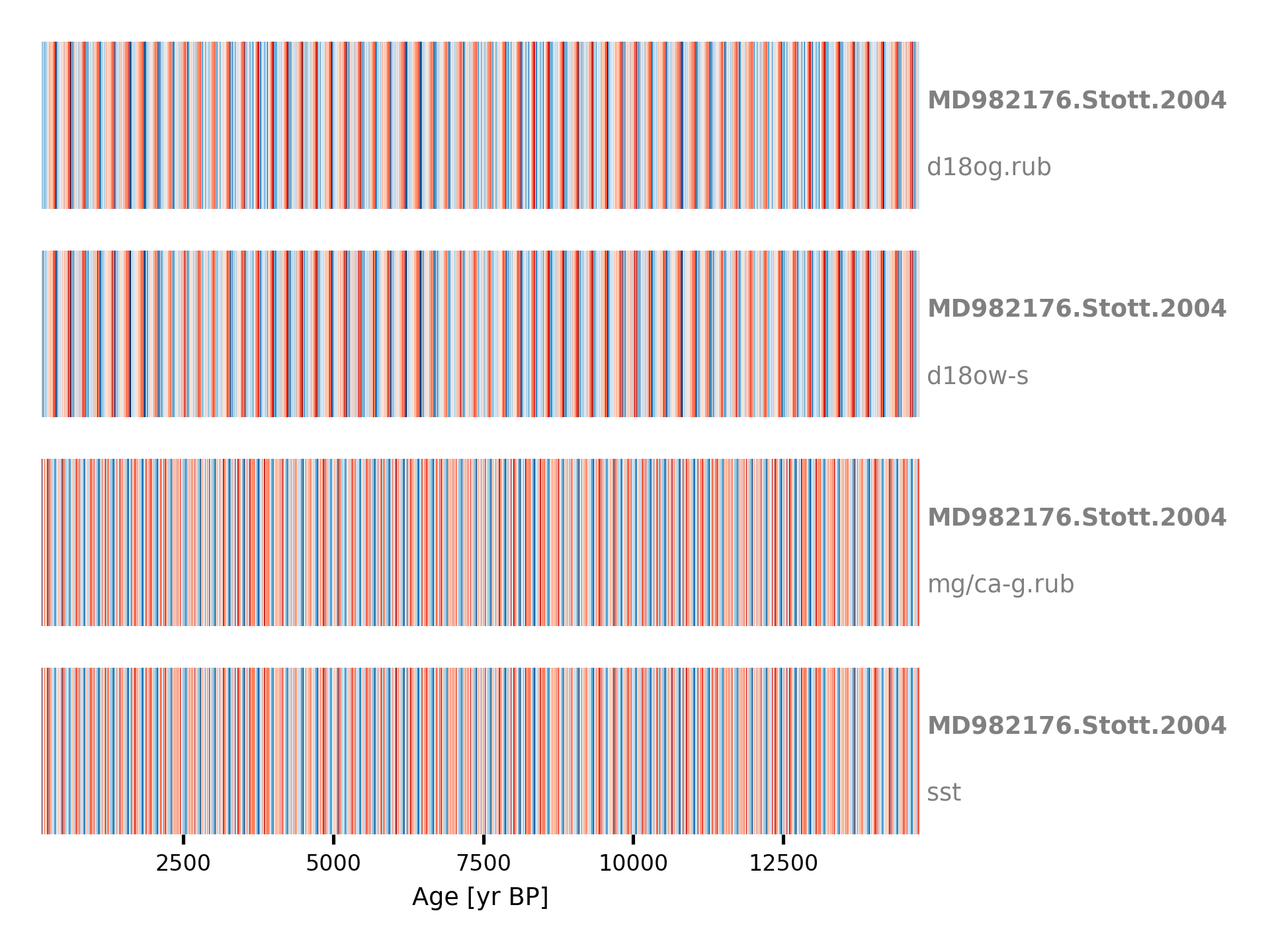
The default style has rather thick bands, intense colors, and too many stripes. The first issue can be solved by passing a figsize tuple; the second by increasing the LIM parameter; the third by passing a step of 0.5 (500y) to common_time(). Finally, the labels are too close to the edge of the plot, which can be adjusted with x_offset, like so:

In [9]: import pyleoclim as pyleo

In [10]: url = 'http://wiki.linked.earth/wiki/index.php/Special:WTLiPD?op=export&lipdid=MD982176.Stott.2004'

In [11]: d = pyleo.Lipd(usr_path = url)
Disclaimer: LiPD files may be updated and modified to adhere to standards

reading: MD982176.Stott.2004.lpd
Finished read: 1 record

In [12]: tslist = d.to_LipdSeriesList()
extracting paleoData...
extracting: MD982176.Stott.2004
Created time series: 6 entries

In [13]: tslist = tslist[2:] # drop the first two series which only concerns age and depth

In [14]: ms = pyleo.MultipleSeries(tslist)

In [15]: fig, ax = ms.stripes(common_time_kwargs={'step': 0.5}, x_offset = 200,
   ....:                      LIM=4, figsize=[8,3])
   ....: 

In [16]: pyleo.closefig(fig)

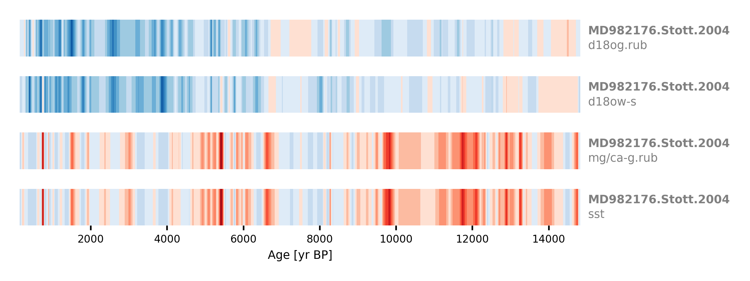
wavelet(method='cwt', settings={}, freq_method='log', freq_kwargs=None, verbose=False, mute_pbar=False)[source]

Wavelet analysis

Parameters:

method (str {wwz, cwt}) –
- cwt - the continuous wavelet transform (as per Torrence and Compo [1998])
  is appropriate only for evenly-spaced series.
- wwz - the weighted wavelet Z-transform (as per Foster [1996])
  is appropriate for both evenly and unevenly-spaced series.
Default is cwt, returning an error if the Series is unevenly-spaced.
settings (dict) – Settings for the particular method. The default is {}.
freq_method (str; {'log', 'scale', 'nfft', 'lomb_scargle', 'welch'}) –
freq_kwargs (dict) – Arguments for frequency vector
settings – Arguments for the specific spectral method
verbose (bool) – If True, will print warning messages if there is any
mute_pbar (bool, optional) – Whether to mute the progress bar. The default is False.

Returns:

scals – A Multiple Scalogram object

Return type:

MultipleScalograms

See also

pyleoclim.utils.wavelet.wwz: wwz function
pyleoclim.utils.wavelet.cwt: cwt function
pyleoclim.utils.wavelet.make_freq_vector: Functions to create the frequency vector
pyleoclim.utils.tsutils.detrend: Detrending function
pyleoclim.core.series.Series.wavelet: wavelet analysis on single object
pyleoclim.core.scalograms.MultipleScalogram: Multiple Scalogram object

References

Torrence, C. and G. P. Compo, 1998: A Practical Guide to Wavelet Analysis. Bull. Amer. Meteor. Soc., 79, 61-78. Python routines available at http://paos.colorado.edu/research/wavelets/

Examples

In [1]: import pyleoclim as pyleo

In [2]: url = 'http://wiki.linked.earth/wiki/index.php/Special:WTLiPD?op=export&lipdid=MD982176.Stott.2004'

In [3]: data = pyleo.Lipd(usr_path = url)
Disclaimer: LiPD files may be updated and modified to adhere to standards

reading: MD982176.Stott.2004.lpd
Finished read: 1 record

In [4]: tslist = data.to_LipdSeriesList()
extracting paleoData...
extracting: MD982176.Stott.2004
Created time series: 6 entries

In [5]: tslist = tslist[2:] # drop the first two series which only contain age and depth

In [6]: ms = pyleo.MultipleSeries(tslist)

In [7]: wav = ms.wavelet(method='wwz')

EnsembleSeries (pyleoclim.EnsembleSeries)

class pyleoclim.core.ensembleseries.EnsembleSeries(series_list)[source]

EnsembleSeries object

The EnsembleSeries object is a child of the MultipleSeries object, that is, a special case of MultipleSeries, aiming for ensembles of similar series. Ensembles usually arise from age modeling or Bayesian calibrations. All members of an EnsembleSeries object are assumed to share identical labels and units.

All methods available for MultipleSeries are available for EnsembleSeries. Some functions were modified for the special case of ensembles. The class enables ensemble-oriented methods for computation (e.g., quantiles) and visualization (e.g., envelope plot) that are unavailable to other classes.

Methods

`append`(ts)	Append timeseries ts to MultipleSeries object
`bin`(**kwargs)	Aligns the time axes of a MultipleSeries object, via binning.
`common_time`([method, step, start, stop, ...])	Aligns the time axes of a MultipleSeries object
`convert_time_unit`([time_unit])	Convert the time units of the object
`copy`()	Copy the object
`correlation`([target, timespan, alpha, ...])	Calculate the correlation between an EnsembleSeries object to a target.
`detrend`([method])	Detrend timeseries
`equal_lengths`()	Test whether all series in object have equal length
`filter`([cutoff_freq, cutoff_scale, method])	Filtering the timeseries in the MultipleSeries object
`flip`([axis])	Flips the Series along one or both axes
`gkernel`(**kwargs)	Aligns the time axes of a MultipleSeries object, via Gaussian kernel.
`histplot`([figsize, title, savefig_settings, ...])	Plots the distribution of the timeseries across ensembles
`increments`([step_style, verbose])	Extract grid properties (start, stop, step) of all the Series objects in a collection.
`interp`(**kwargs)	Aligns the time axes of a MultipleSeries object, via interpolation.
`make_labels`()	Initialization of labels
`pca`([weights, missing, tol_em, max_em_iter])	Principal Component Analysis (Empirical Orthogonal Functions)
`plot`([figsize, marker, markersize, ...])	Plot multiple timeseries on the same axis
`plot_envelope`([figsize, qs, xlabel, ylabel, ...])	Plot EnsembleSeries as an envelope.
`plot_traces`([figsize, xlabel, ylabel, ...])	Plot EnsembleSeries as a subset of traces.
`quantiles`([qs])	Calculate quantiles of an EnsembleSeries object
`slice`(timespan)	Selects a limited time span from the object
`spectral`([method, settings, mute_pbar, ...])	Perform spectral analysis on the timeseries
`stackplot`([figsize, savefig_settings, xlim, ...])	Stack plot of multiple series
`standardize`()	Standardize each series object in a collection
`stripes`([ref_period, figsize, ...])	Represents a MultipleSeries object as a quilt of Ed Hawkins' "stripes" patterns
`wavelet`([method, settings, freq_method, ...])	Wavelet analysis

correlation(target=None, timespan=None, alpha=0.05, settings=None, fdr_kwargs=None, common_time_kwargs=None, mute_pbar=False, seed=None)[source]

Calculate the correlation between an EnsembleSeries object to a target.

If the target is not specified, then the 1st member of the ensemble will be the target Note that the FDR approach is applied by default to determine the significance of the p-values (more information in See Also below).

Parameters:

target (Series or EnsembleSeries) – A pyleoclim Series object or EnsembleSeries object. When the target is also an EnsembleSeries object, then the calculation of correlation is performed in a one-to-one sense, and the ourput list of correlation values and p-values will be the size of the series_list of the self object. That is, if the self object contains n Series, and the target contains n+m Series, then only the first n Series from the object will be used for the calculation; otherwise, if the target contains only n-m Series, then the first m Series in the target will be used twice in sequence.
timespan (tuple) – The time interval over which to perform the calculation
alpha (float) – The significance level (0.05 by default)
settings (dict) –
Parameters for the correlation function, including:

nsimint
the number of simulations (default: 1000)

methodstr, {‘ttest’,’isopersistent’,’isospectral’ (default)}
method for significance testing
fdr_kwargs (dict) – Parameters for the FDR function
common_time_kwargs (dict) – Parameters for the method MultipleSeries.common_time()
mute_pbar (bool; {True,False}) – If True, the progressbar will be muted. Default is False.
seed (float or int) – random seed for isopersistent and isospectral methods

Returns:

corr_ens – The resulting object, see pyleoclim.CorrEns

Return type:

CorrEns

See also

pyleoclim.utils.correlation.corr_sig: Correlation function
pyleoclim.utils.correlation.fdr: False Discovery Rate
pyleoclim.core.correns.CorrEns: The correlation ensemble object

Examples

In [1]: nn = 50 # number of noise realizations

In [2]: nt = 100

In [3]: series_list = []

In [4]: time, signal = pyleo.utils.gen_ts(model='colored_noise',nt=nt,alpha=2.0)

In [5]: ts = pyleo.Series(time=time, value = signal).standardize()

In [6]: noise = np.random.randn(nt,nn)

In [7]: for idx in range(nn):  # noise
   ...:     ts = pyleo.Series(time=time, value=ts.value+5*noise[:,idx])
   ...:     series_list.append(ts)
   ...: 

In [8]: ts_ens = pyleo.EnsembleSeries(series_list)

# set an arbitrary random seed to fix the result
In [9]: corr_res = ts_ens.correlation(ts, seed=2333)
Looping over 50 Series in the ensemble

In [10]: print(corr_res)
  correlation  p-value    signif. w/o FDR (α: 0.05)    signif. w/ FDR (α: 0.05)
-------------  ---------  ---------------------------  --------------------------
0318968  0.75       False                        False
108358   0.23       False                        False
158776   0.08       False                        False
228877   < 1e-2     True                         True
235489   < 1e-2     True                         True
281585   < 1e-6     True                         True
300314   < 1e-6     True                         True
316523   < 1e-6     True                         True
373237   < 1e-6     True                         True
421786   < 1e-6     True                         True
413161   < 1e-6     True                         True
449758   < 1e-6     True                         True
455971   < 1e-6     True                         True
42179    < 1e-6     True                         True
451446   < 1e-6     True                         True
457276   < 1e-6     True                         True
468848   < 1e-6     True                         True
45944    < 1e-6     True                         True
470759   < 1e-6     True                         True
511104   < 1e-6     True                         True
545499   < 1e-6     True                         True
546838   < 1e-6     True                         True
591144   < 1e-6     True                         True
629655   < 1e-6     True                         True
636528   < 1e-6     True                         True
652855   < 1e-6     True                         True
674387   < 1e-6     True                         True
668124   < 1e-6     True                         True
705602   < 1e-6     True                         True
708187   < 1e-6     True                         True
740496   < 1e-6     True                         True
753498   < 1e-6     True                         True
783167   < 1e-6     True                         True
779332   < 1e-6     True                         True
792014   < 1e-6     True                         True
813791   < 1e-6     True                         True
846815   < 1e-6     True                         True
855846   < 1e-6     True                         True
875667   < 1e-6     True                         True
893197   < 1e-6     True                         True
910903   < 1e-6     True                         True
905068   < 1e-6     True                         True
928391   < 1e-6     True                         True
938966   < 1e-6     True                         True
951071   < 1e-6     True                         True
960287   < 1e-6     True                         True
969153   < 1e-6     True                         True
980214   < 1e-6     True                         True
989084   < 1e-6     True                         True
        < 1e-6     True                         True
Ensemble size: 50

The print function tabulates the output, and conveys the p-value according to the correlation test applied (“isospec”, by default). To plot the result:

In [11]: corr_res.plot()
Out[11]: 
(<Figure size 400x400 with 1 Axes>,
 <AxesSubplot: xlabel='$r$', ylabel='Count'>)

In [12]: pyleo.closefig(fig)

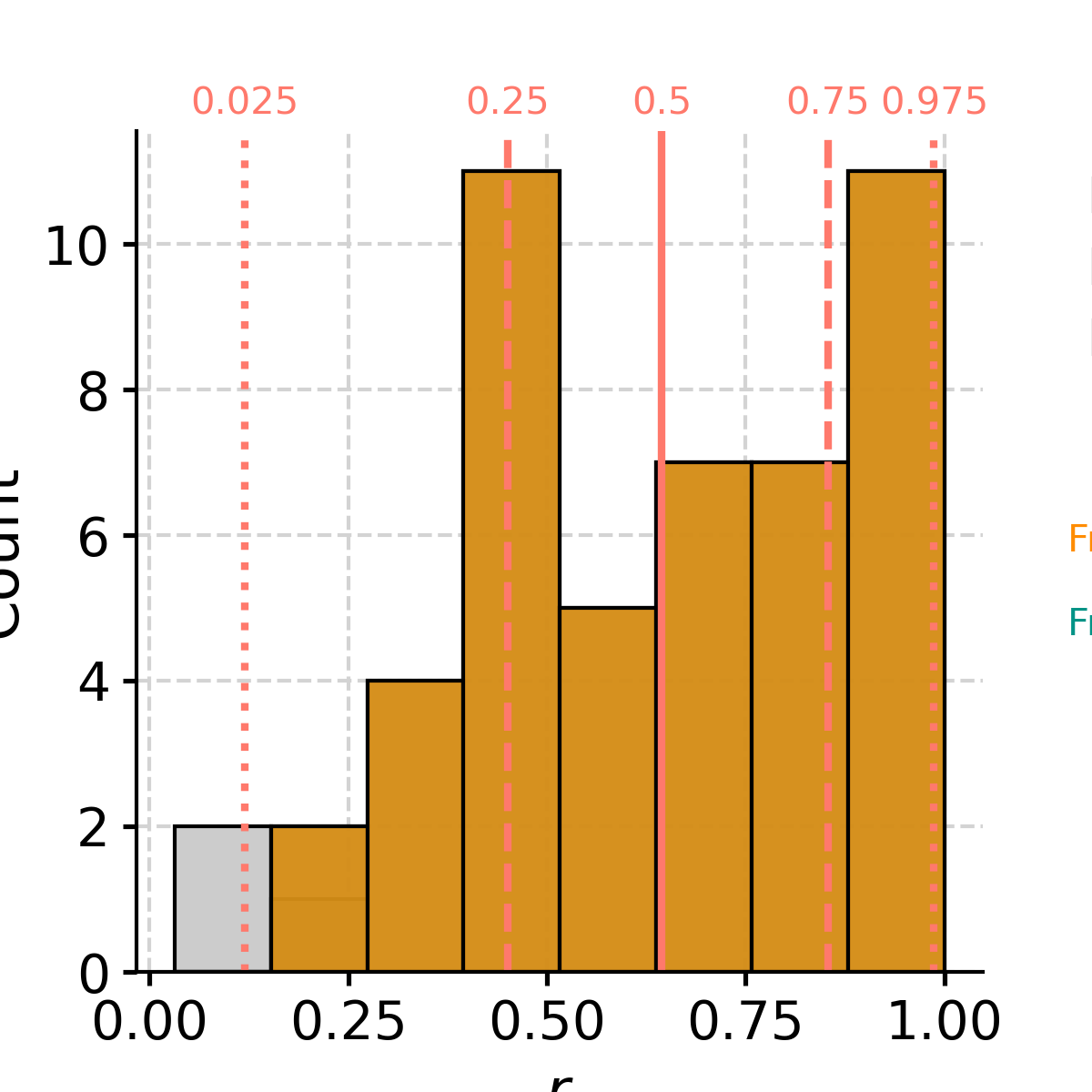
histplot(figsize=[10, 4], title=None, savefig_settings=None, ax=None, ylabel='KDE', vertical=False, edgecolor='w', **plot_kwargs)[source]

Plots the distribution of the timeseries across ensembles

Reuses seaborn [histplot](https://seaborn.pydata.org/generated/seaborn.histplot.html) function.

Parameters:

figsize (list, optional) – The size of the figure. The default is [10, 4].
title (str, optional) – Title for the figure. The default is None.
savefig_settings (dict, optional) –
the dictionary of arguments for plt.savefig(); some notes below:
- ”path” must be specified; it can be any existed or non-existed path, with or without a suffix; if the suffix is not given in “path”, it will follow “format”
- ”format” can be one of {“pdf”, “eps”, “png”, “ps”}.
The default is None.
ax (matplotlib.axis, optional) – A matplotlib axis. The default is None.
ylabel (str, optional) – Label for the count axis. The default is ‘KDE’.
vertical (bool; {True,False}, optional) – Whether to flip the plot vertically. The default is False.
edgecolor (matplotlib.color, optional) – The color of the edges of the bar. The default is ‘w’.
plot_kwargs (dict) – Plotting arguments for seaborn histplot: https://seaborn.pydata.org/generated/seaborn.histplot.html.

See also

pyleoclim.utils.plotting.savefig: Saving figure in Pyleoclim

Examples

In [1]: nn = 30 # number of noise realizations

In [2]: nt = 500

In [3]: series_list = []

In [4]: time, signal = pyleo.utils.gen_ts(model='colored_noise',nt=nt,alpha=1.0)

In [5]: ts = pyleo.Series(time=time, value = signal).standardize()

In [6]: noise = np.random.randn(nt,nn)

In [7]: for idx in range(nn):  # noise
   ...:     ts = pyleo.Series(time=time, value=signal+noise[:,idx])
   ...:     series_list.append(ts)
   ...: 

In [8]: ts_ens = pyleo.EnsembleSeries(series_list)

In [9]: fig, ax = ts_ens.histplot()

In [10]: pyleo.closefig(fig)

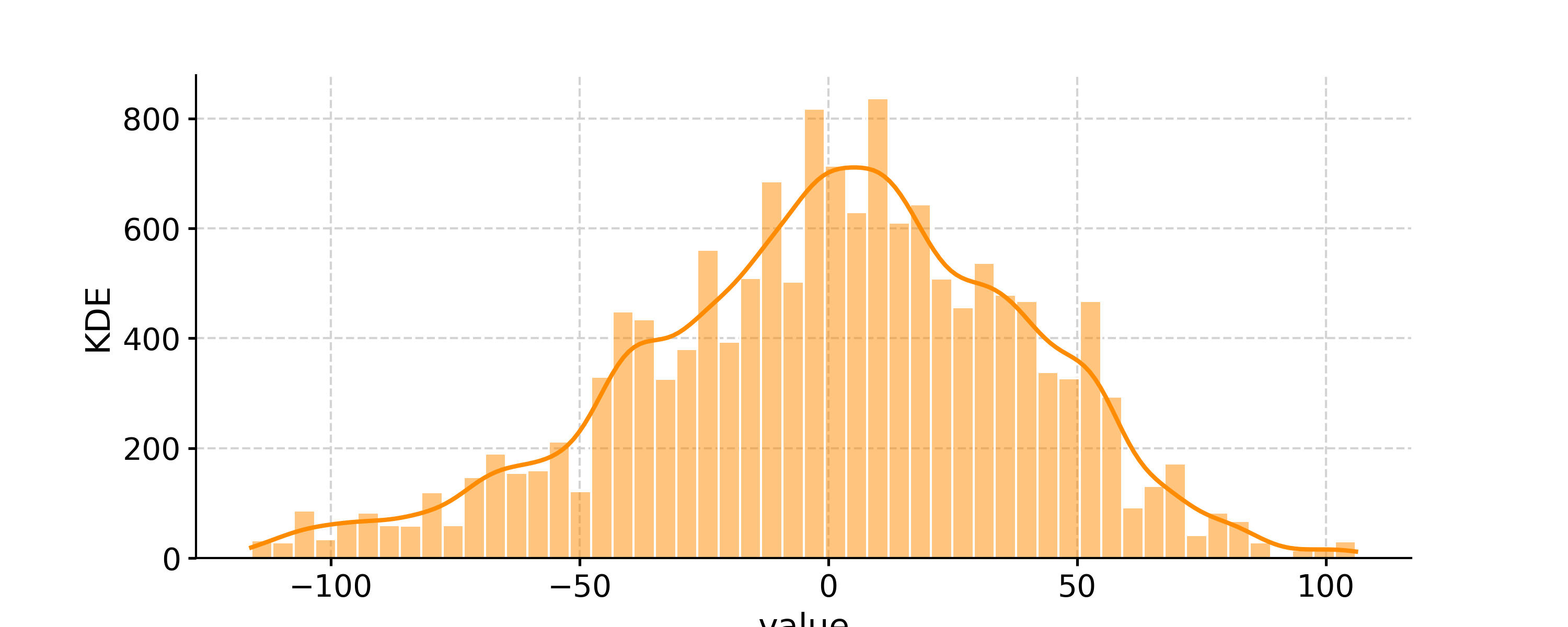
make_labels()[source]

Initialization of labels

Returns:

time_header (str) – Label for the time axis
value_header (str) – Label for the value axis

plot_envelope(figsize=[10, 4], qs=[0.025, 0.25, 0.5, 0.75, 0.975], xlabel=None, ylabel=None, title=None, xlim=None, ylim=None, savefig_settings=None, ax=None, plot_legend=True, curve_clr='#d9544d', curve_lw=2, shade_clr='#d9544d', shade_alpha=0.2, inner_shade_label='IQR', outer_shade_label='95% CI', lgd_kwargs=None)[source]

Plot EnsembleSeries as an envelope.

Parameters:

figsize (list, optional) – The figure size. The default is [10, 4].
qs (list, optional) – The significance levels to consider. The default is [0.025, 0.25, 0.5, 0.75, 0.975] (median, interquartile range, and central 95% region)
xlabel (str, optional) – x-axis label. The default is None.
ylabel (str, optional) – y-axis label. The default is None.
title (str, optional) – Plot title. The default is None.
xlim (list, optional) – x-axis limits. The default is None.
ylim (list, optional) – y-axis limits. The default is None.
savefig_settings (dict, optional) –
the dictionary of arguments for plt.savefig(); some notes below: - “path” must be specified; it can be any existed or non-existed path,

with or without a suffix; if the suffix is not given in “path”, it will follow “format”
- ”format” can be one of {“pdf”, “eps”, “png”, “ps”} The default is None.
ax (matplotlib.ax, optional) – Matplotlib axis on which to return the plot. The default is None.
plot_legend (bool; {True,False}, optional) – Wether to plot the legend. The default is True.
curve_clr (str, optional) – Color of the main line (median). The default is sns.xkcd_rgb[‘pale red’].
curve_lw (str, optional) – Width of the main line (median). The default is 2.
shade_clr (str, optional) – Color of the shaded envelope. The default is sns.xkcd_rgb[‘pale red’].
shade_alpha (float, optional) – Transparency on the envelope. The default is 0.2.
inner_shade_label (str, optional) – Label for the envelope. The default is ‘IQR’.
outer_shade_label (str, optional) – Label for the envelope. The default is ‘95% CI’.
lgd_kwargs (dict, optional) – Parameters for the legend. The default is None.

Returns:

fig (matplotlib.figure) – the figure object from matplotlib See [matplotlib.pyplot.figure](https://matplotlib.org/3.1.1/api/_as_gen/matplotlib.pyplot.figure.html) for details.
ax (matplotlib.axis) – the axis object from matplotlib See [matplotlib.axes](https://matplotlib.org/api/axes_api.html) for details.

See also

pyleoclim.utils.plotting.savefig: Saving figure in Pyleoclim

Examples

In [1]: nn = 30 # number of noise realizations

In [2]: nt = 500

In [3]: series_list = []

In [4]: t,v = pyleo.utils.gen_ts(model='colored_noise',nt=nt,alpha=1.0)

In [5]: signal = pyleo.Series(t,v)

In [6]: for idx in range(nn):  # noise
   ...:     noise = np.random.randn(nt,nn)*100
   ...:     ts = pyleo.Series(time=signal.time, value=signal.value+noise[:,idx])
   ...:     series_list.append(ts)
   ...: 

In [7]: ts_ens = pyleo.EnsembleSeries(series_list)

In [8]: fig, ax = ts_ens.plot_envelope(curve_lw=1.5)

In [9]: pyleo.closefig(fig) #Optional close fig after plotting

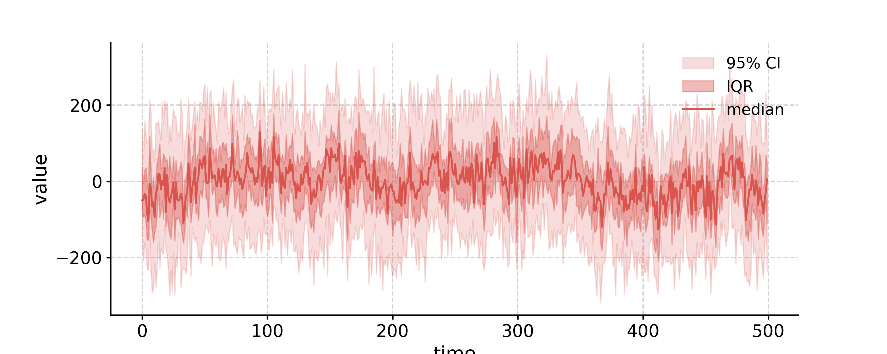
plot_traces(figsize=[10, 4], xlabel=None, ylabel=None, title=None, num_traces=10, seed=None, xlim=None, ylim=None, linestyle='-', savefig_settings=None, ax=None, plot_legend=True, color='#d9544d', lw=0.5, alpha=0.3, lgd_kwargs=None)[source]

Plot EnsembleSeries as a subset of traces.

Parameters:

figsize (list, optional) – The figure size. The default is [10, 4].
xlabel (str, optional) – x-axis label. The default is None.
ylabel (str, optional) – y-axis label. The default is None.
title (str, optional) – Plot title. The default is None.
xlim (list, optional) – x-axis limits. The default is None.
ylim (list, optional) – y-axis limits. The default is None.
color (str, optional) – Color of the traces. The default is sns.xkcd_rgb[‘pale red’].
alpha (float, optional) – Transparency of the lines representing the multiple members. The default is 0.3.
linestyle ({'-', '--', '-.', ':', '', (offset, on-off-seq), ...}) – Set the linestyle of the line
lw (float, optional) – Width of the lines representing the multiple members. The default is 0.5.
num_traces (int, optional) – Number of traces to plot. The default is 10.
savefig_settings (dict, optional) –
the dictionary of arguments for plt.savefig(); some notes below: - “path” must be specified; it can be any existed or non-existed path,

with or without a suffix; if the suffix is not given in “path”, it will follow “format”
- ”format” can be one of {“pdf”, “eps”, “png”, “ps”} The default is None.
ax (matplotlib.ax, optional) – Matplotlib axis on which to return the plot. The default is None.
plot_legend (bool; {True,False}, optional) – Whether to plot the legend. The default is True.
lgd_kwargs (dict, optional) – Parameters for the legend. The default is None.
seed (int, optional) – Set the seed for the random number generator. Useful for reproducibility. The default is None.

Returns:

fig (matplotlib.figure) – the figure object from matplotlib See [matplotlib.pyplot.figure](https://matplotlib.org/3.1.1/api/_as_gen/matplotlib.pyplot.figure.html) for details.
ax (matplotlib.axis) – the axis object from matplotlib See [matplotlib.axes](https://matplotlib.org/api/axes_api.html) for details.

See also

pyleoclim.utils.plotting.savefig: Saving figure in Pyleoclim

Examples

In [1]: nn = 30 # number of noise realizations

In [2]: nt = 500

In [3]: series_list = []

In [4]: t,v = pyleo.utils.gen_ts(model='colored_noise',nt=nt,alpha=1.0)

In [5]: signal = pyleo.Series(t,v)

In [6]: for idx in range(nn):  # noise
   ...:     noise = np.random.randn(nt,nn)*100
   ...:     ts = pyleo.Series(time=signal.time, value=signal.value+noise[:,idx])
   ...:     series_list.append(ts)
   ...: 

In [7]: ts_ens = pyleo.EnsembleSeries(series_list)

In [8]: fig, ax = ts_ens.plot_traces(alpha=0.2,num_traces=8)

In [9]: pyleo.closefig(fig) #Optional close fig after plotting

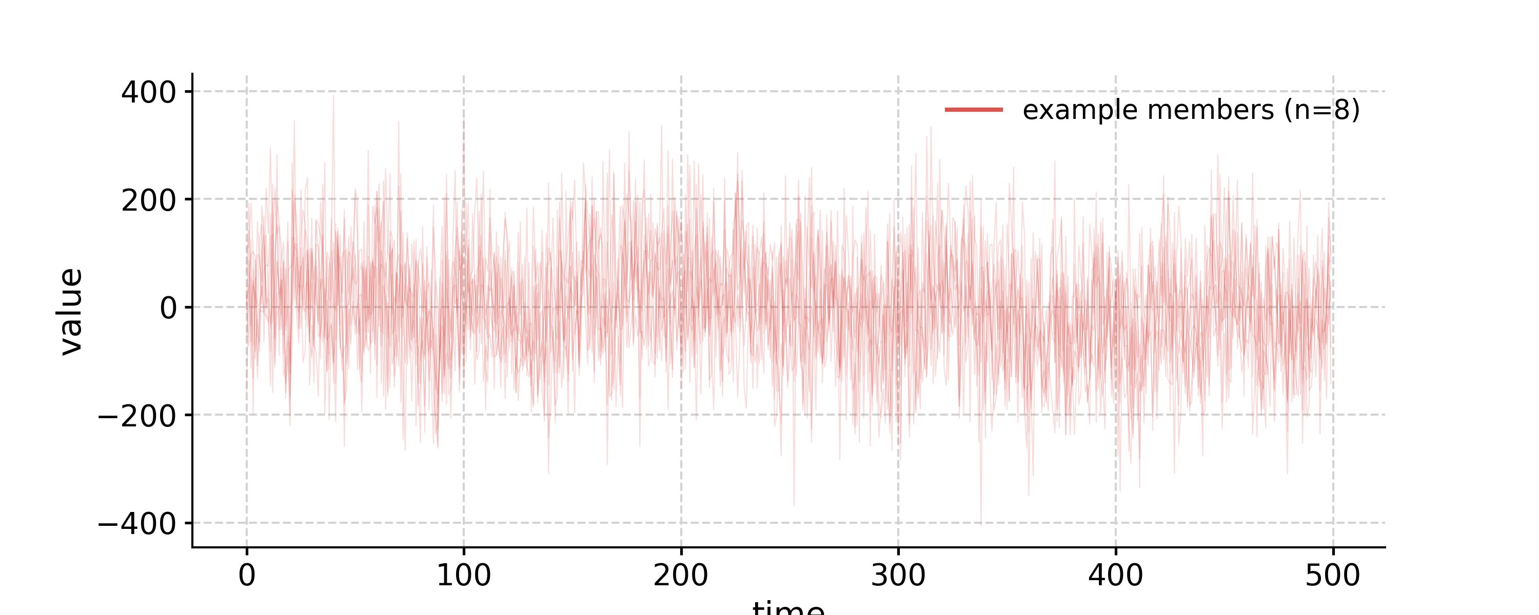
quantiles(qs=[0.05, 0.5, 0.95])[source]

Calculate quantiles of an EnsembleSeries object

Reuses [scipy.stats.mstats.mquantiles](https://docs.scipy.org/doc/scipy/reference/generated/scipy.stats.mstats.mquantiles.html) function.

Parameters:: qs (list, optional) – List of quantiles to consider for the calculation. The default is [0.05, 0.5, 0.95].
Returns:: ens_qs – EnsembleSeries object containing empirical quantiles of original
Return type:: EnsembleSeries

Examples

In [1]: nn = 30 # number of noise realizations

In [2]: nt = 500

In [3]: series_list = []

In [4]: t,v = pyleo.utils.gen_ts(model='colored_noise',nt=nt,alpha=1.0)

In [5]: signal = pyleo.Series(t,v)

In [6]: for idx in range(nn):  # noise
   ...:     noise = np.random.randn(nt,nn)*100
   ...:     ts = pyleo.Series(time=signal.time, value=signal.value+noise[:,idx])
   ...:     series_list.append(ts)
   ...: 

In [7]: ts_ens = pyleo.EnsembleSeries(series_list)

In [8]: ens_qs = ts_ens.quantiles()

slice(timespan)[source]

Selects a limited time span from the object

Parameters:: timespan (tuple or list) – The list of time points for slicing, whose length must be even. When there are n time points, the output Series includes n/2 segments. For example, if timespan = [a, b], then the sliced output includes one segment [a, b]; if timespan = [a, b, c, d], then the sliced output includes segment [a, b] and segment [c, d].
Returns:: new – The sliced EnsembleSeries object.
Return type:: EnsembleSeries

Examples

slice the SOI from 1972 to 1998

In [1]: nn = 20 # number of noise realizations

In [2]: nt = 200

In [3]: series_list = []

In [4]: time, signal = pyleo.utils.gen_ts(model='colored_noise',nt=nt,alpha=2.0)

In [5]: ts = pyleo.Series(time=time, value = signal).standardize()

In [6]: noise = np.random.randn(nt,nn)

In [7]: for idx in range(nn):  # noise
   ...:     ts = pyleo.Series(time=time, value=ts.value+5*noise[:,idx])
   ...:     series_list.append(ts)
   ...: 

In [8]: ts_ens = pyleo.EnsembleSeries(series_list)

In [9]: fig, ax = ts_ens.plot_envelope(curve_lw=1.5)

In [10]: fig, ax = ts_ens.slice([100, 199]).plot_envelope(curve_lw=1.5)

In [11]: pyleo.closefig(fig)

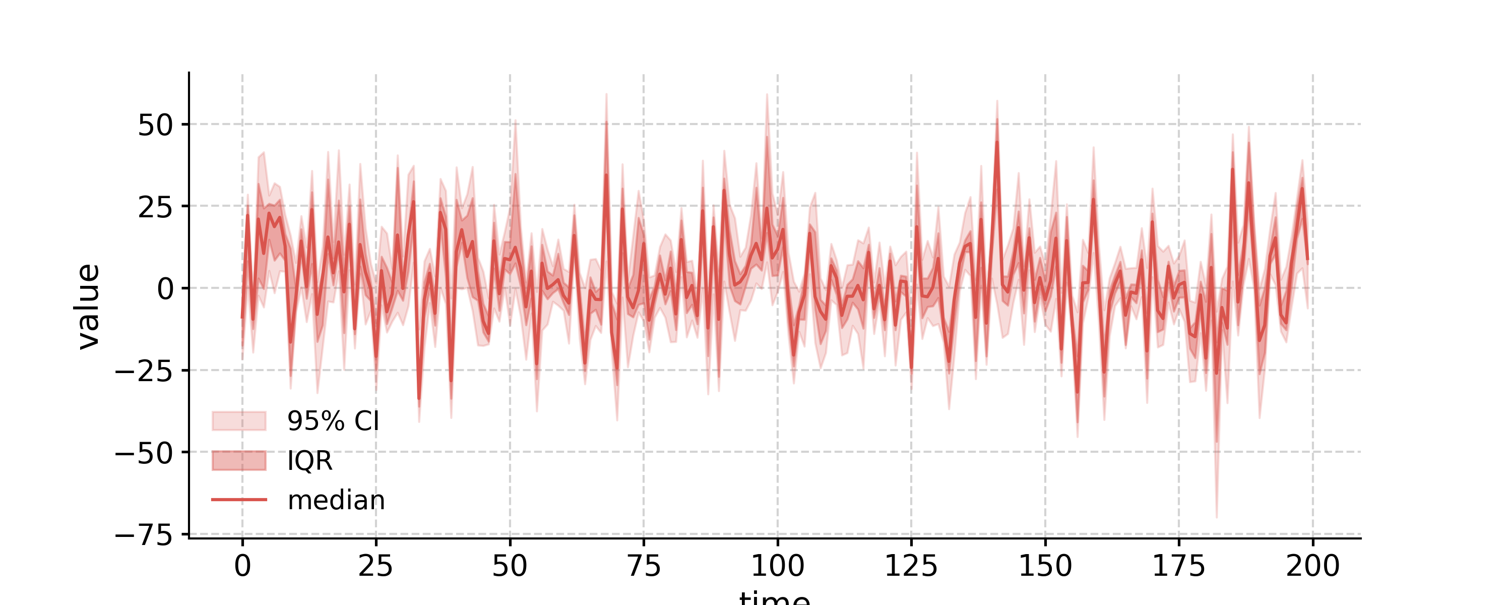
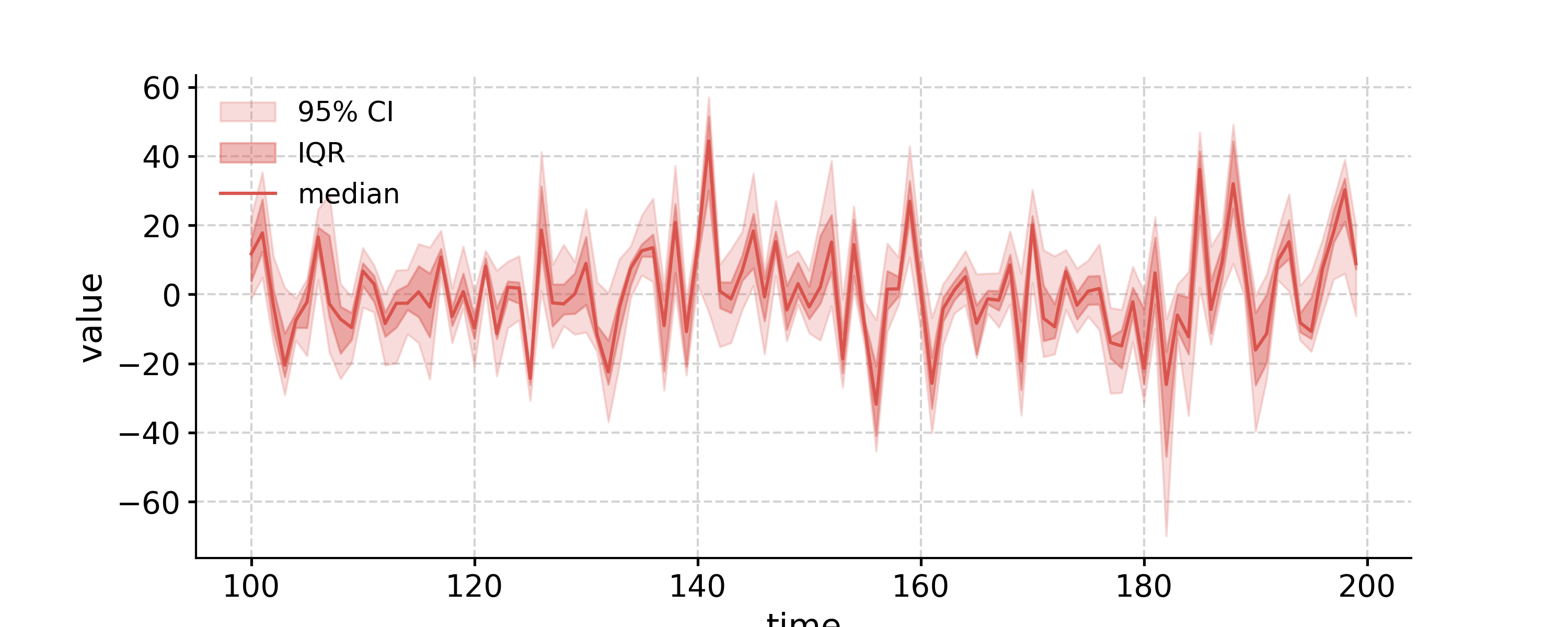
stackplot(figsize=[5, 15], savefig_settings=None, xlim=None, fill_between_alpha=0.2, colors=None, cmap='tab10', norm=None, spine_lw=1.5, grid_lw=0.5, font_scale=0.8, label_x_loc=-0.15, v_shift_factor=0.75, linewidth=1.5)[source]

Stack plot of multiple series

Note that the plotting style is uniquely designed for this one and cannot be properly reset with pyleoclim.set_style().

Parameters:

figsize (list) – Size of the figure.
colors (list) – Colors for plotting. If None, the plotting will cycle the ‘tab10’ colormap; if only one color is specified, then all curves will be plotted with that single color; if a list of colors are specified, then the plotting will cycle that color list.
cmap (str) – The colormap to use when “colors” is None.
norm (matplotlib.colors.Normalize like) – The nomorlization for the colormap. If None, a linear normalization will be used.
savefig_settings (dictionary) –
the dictionary of arguments for plt.savefig(); some notes below: - “path” must be specified; it can be any existed or non-existed path,

with or without a suffix; if the suffix is not given in “path”, it will follow “format”
- ”format” can be one of {“pdf”, “eps”, “png”, “ps”} The default is None.
xlim (list) – The x-axis limit.
fill_between_alpha (float) – The transparency for the fill_between shades.
spine_lw (float) – The linewidth for the spines of the axes.
grid_lw (float) – The linewidth for the gridlines.
linewidth (float) – The linewidth for the curves.
font_scale (float) – The scale for the font sizes. Default is 0.8.
label_x_loc (float) – The x location for the label of each curve.
v_shift_factor (float) – The factor for the vertical shift of each axis. The default value 3/4 means the top of the next axis will be located at 3/4 of the height of the previous one.

Returns:

fig (matplotlib.figure) – the figure object from matplotlib See [matplotlib.pyplot.figure](https://matplotlib.org/3.1.1/api/_as_gen/matplotlib.pyplot.figure.html) for details.
ax (matplotlib.axis) – the axis object from matplotlib See [matplotlib.axes](https://matplotlib.org/api/axes_api.html) for details.

See also

pyleoclim.utils.plotting.savefig: Saving figure in Pyleoclim

Examples

In [1]: nn = 10 # number of noise realizations

In [2]: nt = 200

In [3]: series_list = []

In [4]: t, v = pyleo.utils.gen_ts(model='colored_noise',nt=nt,alpha=1.0)

In [5]: signal, _, _ = pyleo.utils.standardize(v)

In [6]: noise = np.random.randn(nt,nn)

In [7]: for idx in range(nn):  # noise
   ...:     ts = pyleo.Series(time=t, value=signal+noise[:,idx], label='trace #'+str(idx+1))
   ...:     series_list.append(ts)
   ...: 

In [8]: ts_ens = pyleo.EnsembleSeries(series_list)

In [9]: fig, ax = ts_ens.stackplot()

In [10]: pyleo.closefig(fig) #Optional close fig after plotting

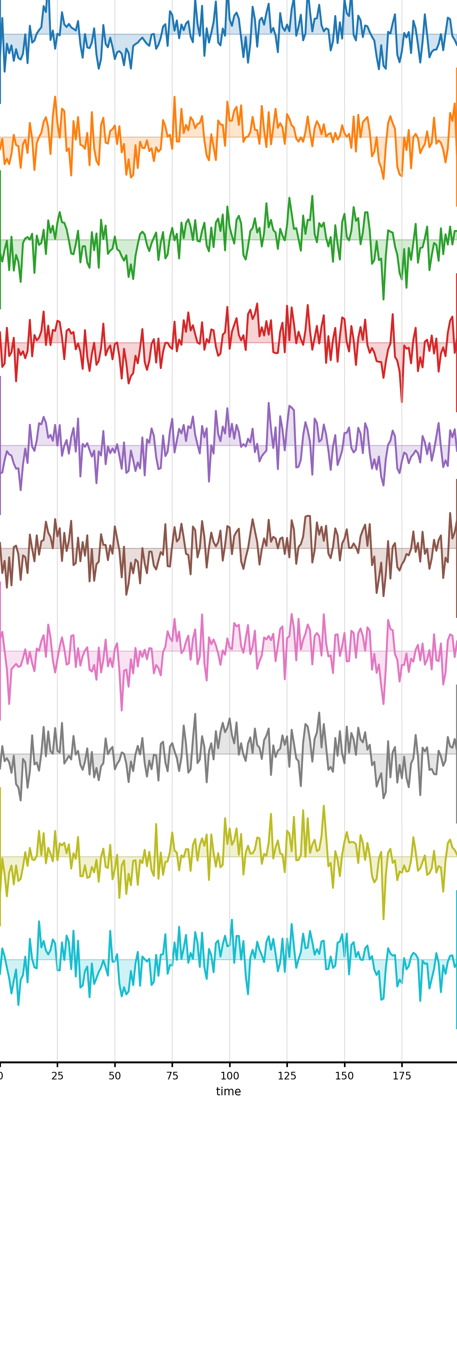
SurrogateSeries (pyleoclim.SurrogateSeries)

class pyleoclim.core.surrogateseries.SurrogateSeries(series_list, surrogate_method=None, surrogate_args=None)[source]

Object containing surrogate timeseries, usually obtained through recursive modeling (e.g., AR1)

Surrogate Series is a child of MultipleSeries. All methods available for MultipleSeries are available for surrogate series.

Methods

`append`(ts)	Append timeseries ts to MultipleSeries object
`bin`(**kwargs)	Aligns the time axes of a MultipleSeries object, via binning.
`common_time`([method, step, start, stop, ...])	Aligns the time axes of a MultipleSeries object
`convert_time_unit`([time_unit])	Convert the time units of the object
`copy`()	Copy the object
`correlation`([target, timespan, alpha, ...])	Calculate the correlation between a MultipleSeries and a target Series
`detrend`([method])	Detrend timeseries
`equal_lengths`()	Test whether all series in object have equal length
`filter`([cutoff_freq, cutoff_scale, method])	Filtering the timeseries in the MultipleSeries object
`flip`([axis])	Flips the Series along one or both axes
`gkernel`(**kwargs)	Aligns the time axes of a MultipleSeries object, via Gaussian kernel.
`increments`([step_style, verbose])	Extract grid properties (start, stop, step) of all the Series objects in a collection.
`interp`(**kwargs)	Aligns the time axes of a MultipleSeries object, via interpolation.
`pca`([weights, missing, tol_em, max_em_iter])	Principal Component Analysis (Empirical Orthogonal Functions)
`plot`([figsize, marker, markersize, ...])	Plot multiple timeseries on the same axis
`spectral`([method, settings, mute_pbar, ...])	Perform spectral analysis on the timeseries
`stackplot`([figsize, savefig_settings, xlim, ...])	Stack plot of multiple series
`standardize`()	Standardize each series object in a collection
`stripes`([ref_period, figsize, ...])	Represents a MultipleSeries object as a quilt of Ed Hawkins' "stripes" patterns
`wavelet`([method, settings, freq_method, ...])	Wavelet analysis

Lipd (pyleoclim.Lipd)

This class allows to manipulate LiPD objects.

class pyleoclim.core.lipd.Lipd(usr_path=None, lipd_dict=None, validate=False, remove=False)[source]

The Lipd class allows to create a Lipd object from Lipd files. This allows to manipulate LiPD objects and take advantage of the metadata information for specific functionalities. Lipd objects are needed to create LipdSeries objects, which carry most of the timeseries functionalities.

Parameters:

usr_path (str) – Path to the Lipd file(s). Can be URL (LiPD utilities only support loading one file at a time from a URL). If it’s a URL, it must start with “http”, “https”, or “ftp”.
lidp_dict (dict) – LiPD files already loaded into Python through the LiPD utilities
validate (bool) – Validate the LiPD files upon loading. Note that for a large library (>300files) this can take up to half an hour.
remove (bool) – If validate is True and remove is True, ignores non-valid LiPD files. Note that loading unvalidated Lipd files may result in errors for some functionalities but not all.

References

McKay, N. P., & Emile-Geay, J. (2016). Technical Note: The Linked Paleo Data framework – a common tongue for paleoclimatology. Climate of the Past, 12, 1093-1100.

Examples

In [1]: import pyleoclim as pyleo

In [2]: url='http://wiki.linked.earth/wiki/index.php/Special:WTLiPD?op=export&lipdid=MD982176.Stott.2004'

In [3]: d=pyleo.Lipd(usr_path=url)
Disclaimer: LiPD files may be updated and modified to adhere to standards

reading: MD982176.Stott.2004.lpd
Finished read: 1 record

Methods

`copy`()	Copy the object
`extract`(dataSetName)	param dataSetName: Extract a particular dataset
`mapAllArchive`([projection, proj_default, ...])	Map all the records contained in the LiPD object by the type of archive
`to_LipdSeries`([number, mode])	Extracts one timeseries from the Lipd object
`to_LipdSeriesList`([mode])	Extracts all LiPD timeseries objects to a list of LipdSeries objects
`to_tso`([mode])	Extracts all the variables to a list of LiPD timeseries objects

copy()[source]: Copy the object

extract(dataSetName)[source]

Parameters:: dataSetName (str) – Extract a particular dataset
Returns:: new – A new object corresponding to a particular dataset
Return type:: Lipd

mapAllArchive(projection='Robinson', proj_default=True, background=True, borders=False, rivers=False, lakes=False, figsize=None, ax=None, marker=None, color=None, markersize=None, scatter_kwargs=None, legend=True, lgd_kwargs=None, savefig_settings=None)[source]

Map all the records contained in the LiPD object by the type of archive

Note that the map is fully cusomizable by using the optional parameters.

Parameters:

projection (str, optional) – The projection to use. The default is ‘Robinson’.
proj_default (bool, optional) – Wether to use the Pyleoclim defaults for each projection type. The default is True.
background (bool, optional) – Wether to use a backgound. The default is True.
borders (bool, optional) – Draw borders. The default is False.
rivers (bool, optional) – Draw rivers. The default is False.
lakes (bool, optional) – Draw lakes. The default is False.
figsize (list, optional) – The size of the figure. The default is None.
ax (matplotlib.ax, optional) – The matplotlib axis onto which to return the map. The default is None.
marker (str, optional) – The marker type for each archive. The default is None, which uses a pre-defined palette in Pyleoclim. To see the default option, run Lipd.plot_default where Lipd is the name of the object.
color (str, optional) – Color for each acrhive. The default is None. The default is None, which uses a pre-defined palette in Pyleoclim. To see the default option, run Lipd.plot_default where Lipd is the name of the object.
markersize (float, optional) – Size of the marker. The default is None.
scatter_kwargs (dict, optional) – Parameters for the scatter plot. The default is None.
legend (bool; {True,False}, optional) – Whether to plot the legend. The default is True.
lgd_kwargs (dict, optional) – Arguments for the legend. The default is None.
savefig_settings (dictionary, optional) –
The dictionary of arguments for plt.savefig(); some notes below: - “path” must be specified; it can be any existing or non-existing path,

with or without a suffix; if the suffix is not given in “path”, it will follow “format”
- ”format” can be one of {“pdf”, “eps”, “png”, “ps”}.
The default is None.

Returns:

res – The figure and axis if asked.

Return type:

tuple or fig

See also

pyleoclim.utils.mapping.map: Underlying mapping function for Pyleoclim

Examples

For speed, we are only using one LiPD file. But these functions can load and map multiple.

In [1]: import pyleoclim as pyleo

In [2]: url = 'http://wiki.linked.earth/wiki/index.php/Special:WTLiPD?op=export&lipdid=MD982176.Stott.2004'

In [3]: data = pyleo.Lipd(usr_path = url)
Disclaimer: LiPD files may be updated and modified to adhere to standards

reading: MD982176.Stott.2004.lpd
Finished read: 1 record

In [4]: fig, ax = data.mapAllArchive()

In [5]: pyleo.closefig(fig)

Change the markersize

In [6]: import pyleoclim as pyleo

In [7]: url = 'http://wiki.linked.earth/wiki/index.php/Special:WTLiPD?op=export&lipdid=MD982176.Stott.2004'

In [8]: data = pyleo.Lipd(usr_path = url)
Disclaimer: LiPD files may be updated and modified to adhere to standards

reading: MD982176.Stott.2004.lpd
Finished read: 1 record

In [9]: fig, ax = data.mapAllArchive(markersize=100)

In [10]: pyleo.closefig(fig)

to_LipdSeries(number=None, mode='paleo')[source]

Extracts one timeseries from the Lipd object

In LiPD, timeseries objects are flatten dictionaries that contain the values for the time and variable axes as well as relevant metadata. Note that this function may require user interaction if the number of the column in the file is unknown. The numbers are fixed so automating the code is as simple as retaining a series of numbers when reopening the files.

Parameters:

number (int) – the number of the timeseries object
mode (str; {'paleo','chron'}) – whether to extract the paleo or chron series.

Returns:

ts – A LipdSeries object

Return type:

pyleoclim.LipdSeries

See also

pyleoclim.core.lipdseries.LipdSeries: LipdSeries object

to_LipdSeriesList(mode='paleo')[source]

Extracts all LiPD timeseries objects to a list of LipdSeries objects

In LiPD, timeseries objects are flatten dictionaries that contain the values for the time and variable axes as well as relevant metadata.

Parameters:: mode ({'paleo','chron'}) – Whether to extract the timeseries information from the paleo tables or chron tables
Returns:: res – A list of LiPDSeries objects
Return type:: list

References

McKay, N. P., & Emile-Geay, J. (2016). Technical Note: The Linked Paleo Data framework – a common tongue for paleoclimatology. Climate of the Past, 12, 1093-1100.

See also

pyleoclim.core.lipdseries.LipdSeries: a LipdSeries object

to_tso(mode='paleo')[source]

Extracts all the variables to a list of LiPD timeseries objects

In LiPD, timeseries objects are flatten dictionaries that contain the values for the time and variable axes as well as relevant metadata.

Parameters:: mode ({'paleo','chron'}) – Whether to extract the timeseries information from the paleo tables or chron tables
Returns:: ts_list – List of LiPD timeseries objects
Return type:: list

References

McKay, N. P., & Emile-Geay, J. (2016). Technical Note: The Linked Paleo Data framework – a common tongue for paleoclimatology. Climate of the Past, 12, 1093-1100.

LipdSeries (pyleoclim.LipdSeries)

class pyleoclim.core.lipdseries.LipdSeries(tso, clean_ts=True, verbose=False)[source]

LipdSeries are (you guessed it), Series objects that are created from LiPD objects. As a subclass of Series, they inherit all its methods. When created, LiPDSeries automatically instantiates the time, value and other parameters from what’s in the lipd file. These objects can be obtained from a LiPD file/object either through Pyleoclim or the LiPD utilities. If multiple objects (i.e., a list) are given, then the user will be prompted to choose one timeseries.

Returns:: object
Return type:: pyleoclim.LipdSeries

See also

pyleoclim.core.lipd.Lipd: Creates a Lipd object from LiPD Files
pyleoclim.core.series.Series: Creates pyleoclim Series object
pyleoclim.core.multipleseries.MultipleSeries: a collection of multiple Series objects

Examples

In this example, we will import a LiPD file and explore the various options to create a series object.

First, let’s look at the Lipd.to_tso option. This method is attractive because the object is a list of dictionaries that are easily explored in Python.

In [1]: import pyleoclim as pyleo

In [2]: url = 'http://wiki.linked.earth/wiki/index.php/Special:WTLiPD?op=export&lipdid=MD982176.Stott.2004'

In [3]: data = pyleo.Lipd(usr_path = url)
Disclaimer: LiPD files may be updated and modified to adhere to standards

reading: MD982176.Stott.2004.lpd
Finished read: 1 record

In [4]: ts_list = data.to_tso()
extracting paleoData...
extracting: MD982176.Stott.2004
Created time series: 6 entries

# Print out the dataset name and the variable name
In [5]: for item in ts_list:
   ...:     print(item['dataSetName']+': '+item['paleoData_variableName'])
   ...: 
MD982176.Stott.2004: depth
MD982176.Stott.2004: yrbp
MD982176.Stott.2004: d18og.rub
MD982176.Stott.2004: d18ow-s
MD982176.Stott.2004: mg/ca-g.rub
MD982176.Stott.2004: sst

# Load the sst data into a LipdSeries. Since Python indexing starts at zero, sst has index 5.
In [6]: ts = pyleo.LipdSeries(ts_list[5])

If you attempt to pass the full list of series, Pyleoclim will prompt you to choose a series by printing out something similar as above. If you already now the number of the timeseries object you’re interested in, then you should use the following:

In [7]: ts1 = data.to_LipdSeries(number=5)
extracting paleoData...
extracting: MD982176.Stott.2004
Created time series: 6 entries

If number is not specified, Pyleoclim will prompt you for the number automatically.

Sometimes, one may want to create a MultipleSeries object from a collection of LiPD files. In this case, we recommend using the following:

In [8]: ts_list = data.to_LipdSeriesList()
extracting paleoData...
extracting: MD982176.Stott.2004
Created time series: 6 entries

# only keep the Mg/Ca and SST
In [9]: ts_list=ts_list[4:]

#create a MultipleSeries object
In [10]: ms=pyleo.MultipleSeries(ts_list)

Methods

`bin`([keep_log])	Bin values in a time series
`causality`(target_series[, method, timespan, ...])	Perform causality analysis with the target timeseries. Specifically, whether there is information in the target series that influenced the original series.
`center`([timespan, keep_log])	Centers the series (i.e.
`chronEnsembleToPaleo`(D[, number, ...])	Fetch chron ensembles from a Lipd object and return the ensemble as MultipleSeries
`clean`([verbose, keep_log])	Clean up the timeseries by removing NaNs and sort with increasing time points
`convert_time_unit`([time_unit, keep_log])	Convert the time unit of the Series object
`copy`()	Copy the object
`correlation`(target_series[, timespan, ...])	Estimates the Pearson's correlation and associated significance between two non IID time series
`dashboard`([figsize, plt_kwargs, ...])	param figsize: Figure size. The default is [11,8].
`detrend`([method, keep_log])	Detrend Series object
`fill_na`([timespan, dt, keep_log])	Fill NaNs into the timespan
`filter`([cutoff_freq, cutoff_scale, method, ...])	Filtering methods for Series objects using four possible methods:
`flip`([axis, keep_log])	Flips the Series along one or both axes
`gaussianize`([keep_log])	Gaussianizes the timeseries (i.e.
`getMetadata`()	Get the necessary metadata for the ensemble plots
`gkernel`([step_type, keep_log])	Coarse-grain a Series object via a Gaussian kernel.
`histplot`([figsize, title, savefig_settings, ...])	Plot the distribution of the timeseries values
`interp`([method, keep_log])	Interpolate a Series object onto a new time axis
`is_evenly_spaced`([tol])	Check if the Series time axis is evenly-spaced, within tolerance
`make_labels`()	Initialization of plot labels based on Series metadata
`map`([projection, proj_default, background, ...])	Map the location of the record
`mapNearRecord`(D[, n, radius, sameArchive, ...])	Map records that are near the timeseries of interest
`outliers`([method, remove, settings, ...])	Remove outliers from timeseries data
`plot`([figsize, marker, markersize, color, ...])	Plot the timeseries
`plot_age_depth`([figsize, plt_kwargs, ...])	param figsize: Size of the figure. The default is [10,4].
`segment`([factor])	Gap detection
`slice`(timespan)	Slicing the timeseries with a timespan (tuple or list)
`sort`([verbose, keep_log])	Ensure timeseries is aligned to a prograde axis.
`spectral`([method, freq_method, freq_kwargs, ...])	Perform spectral analysis on the timeseries
`ssa`([M, nMC, f, trunc, var_thresh])	Singular Spectrum Analysis
`standardize`([keep_log, scale])	Standardizes the series ((i.e.
`stats`()	Compute basic statistics from a Series
`stripes`(ref_period[, LIM, thickness, ...])	Represents the Series as an Ed Hawkins "stripes" pattern
`summary_plot`(psd, scalogram[, figsize, ...])	Produce summary plot of timeseries.
`surrogates`([method, number, length, seed, ...])	Generate surrogates with increasing time axis
`wavelet`([method, settings, freq_method, ...])	Perform wavelet analysis on a timeseries
`wavelet_coherence`(target_series[, method, ...])	Performs wavelet coherence analysis with the target timeseries

chronEnsembleToPaleo(D, number=None, chronNumber=None, modelNumber=None, tableNumber=None)[source]

Fetch chron ensembles from a Lipd object and return the ensemble as MultipleSeries

Parameters:

D (a LiPD object) –
number (int, optional) – The number of ensemble members to store. Default is None, which corresponds to all present
chronNumber (int, optional) – The chron object number. The default is None.
modelNumber (int, optional) – Age model number. The default is None.
tableNumber (int, optional) – Table number. The default is None.

Raises:

ValueError –

Returns:

ens – An EnsembleSeries object with each series representing a possible realization of the age model

Return type:

EnsembleSeries

See also

pyleoclim.core.ensembleseries.EnsembleSeries: An EnsembleSeries object with each series representing a possible realization of the age model
pyleoclim.utils.lipdutils.mapAgeEnsembleToPaleoData: Map the depth for the ensemble age values to the paleo depth

copy()[source]

Copy the object

Returns:: object – New object with data copied from original
Return type:: pyleoclim.LipdSeries

dashboard(figsize=[11, 8], plt_kwargs=None, histplt_kwargs=None, spectral_kwargs=None, spectralsignif_kwargs=None, spectralfig_kwargs=None, map_kwargs=None, metadata=True, savefig_settings=None, ensemble=False, D=None)[source]

Parameters:

figsize (list or tuple, optional) – Figure size. The default is [11,8].
plt_kwargs (dict, optional) – Optional arguments for the timeseries plot. See Series.plot() or EnsembleSeries.plot_envelope(). The default is None.
histplt_kwargs (dict, optional) – Optional arguments for the distribution plot. See Series.histplot() or EnsembleSeries.plot_distplot(). The default is None.
spectral_kwargs (dict, optional) – Optional arguments for the spectral method. Default is to use Lomb-Scargle method. See Series.spectral() or EnsembleSeries.spectral(). The default is None.
spectralsignif_kwargs (dict, optional) – Optional arguments to estimate the significance of the power spectrum. See PSD.signif_test. Note that we currently do not support significance testing for ensembles. The default is None.
spectralfig_kwargs (dict, optional) – Optional arguments for the power spectrum figure. See PSD.plot() or MultiplePSD.plot_envelope(). The default is None.
map_kwargs (dict, optional) – Optional arguments for the map. See LipdSeries.map(). The default is None.
metadata (bool; {True,False}, optional) – Whether or not to produce a dashboard with printed metadata. The default is True.
savefig_settings (dict, optional) –
the dictionary of arguments for plt.savefig(); some notes below: - “path” must be specified; it can be any existed or non-existed path,

with or without a suffix; if the suffix is not given in “path”, it will follow “format”
- ”format” can be one of {“pdf”, “eps”, “png”, “ps”}.
The default is None.
ensemble (bool; {True, False}, optional) – If True, will return the dashboard in ensemble modes if ensembles are available
D (pyleoclim.Lipd object) – If asking for an ensemble plot, a pyleoclim.Lipd object must be provided

Returns:

fig (matplotlib.figure) – The figure
ax (matplolib.axis) – The axis

See also

pyleoclim.core.series.Series.plot: plot a timeseries
pyleoclim.core.ensembleseries.EnsembleSeries.plot_envelope: Envelope plots for an ensemble
pyleoclim.core.series.Series.histplot: plot a distribution of the timeseries
pyleoclim.core.ensembleseries.EnsembleSeries.histplot: plot a distribution of the timeseries across ensembles
pyleoclim.core.series.Series.spectral: spectral analysis method.
pyleoclim.core.multipleseries.MultipleSeries.spectral: spectral analysis method for multiple series.
pyleoclim.core.psds.PSD.signif_test: significance test for timeseries analysis
pyleoclim.core.psds.PSD.plot: plot power spectrum
pyleoclim.core.psds.MulitplePSD.plot: plot envelope of power spectrum
pyleoclim.core.lipdseries.LipdSeries.map: map location of dataset
pyleoclim.core.lipdseries.LipdSeries.getMetadata: get relevant metadata from the timeseries object
pyleoclim.utils.mapping.map: Underlying mapping function for Pyleoclim

Examples

In [1]: import pyleoclim as pyleo

In [2]: url = 'http://wiki.linked.earth/wiki/index.php/Special:WTLiPD?op=export&lipdid=MD982176.Stott.2004'

In [3]: data = pyleo.Lipd(usr_path = url)
Disclaimer: LiPD files may be updated and modified to adhere to standards

reading: MD982176.Stott.2004.lpd
Finished read: 1 record

In [4]: ts = data.to_LipdSeries(number=5)
extracting paleoData...
extracting: MD982176.Stott.2004
Created time series: 6 entries

In [5]: fig, ax = ts.dashboard()

In [6]: pyleo.closefig(fig)

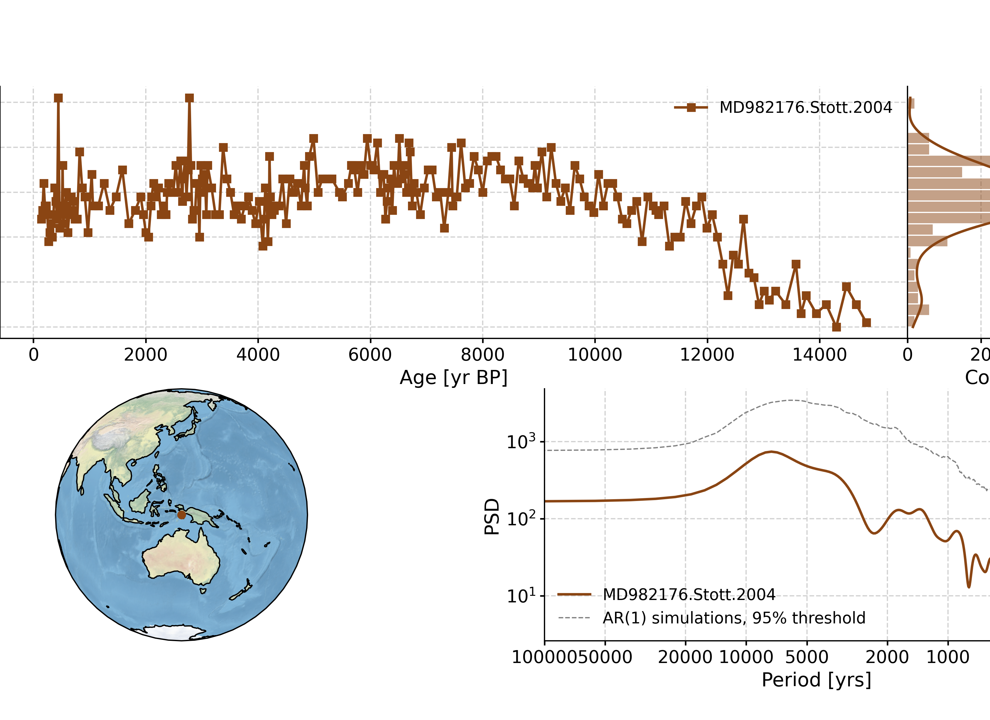
getMetadata()[source]

Get the necessary metadata for the ensemble plots

Parameters:

timeseries (object) – a specific timeseries object.

Returns:

res –

A dictionary containing the following metadata:: archiveType, Authors (if more than 2, replace by et al), PublicationYear, Publication DOI, Variable Name, Units, Climate Interpretation, Calibration Equation, Calibration References, Calibration Notes

Return type:

dict

map(projection='Orthographic', proj_default=True, background=True, borders=False, rivers=False, lakes=False, figsize=None, ax=None, marker=None, color=None, markersize=None, scatter_kwargs=None, legend=True, lgd_kwargs=None, savefig_settings=None)[source]

Map the location of the record

Parameters:

projection (str, optional) – The projection to use. The default is ‘Robinson’.
proj_default (bool; {True, False}, optional) – Whether to use the Pyleoclim defaults for each projection type. The default is True.
background (bool; {True, False}, optional) – Whether to use a background. The default is True.
borders (bool; {True, False}, optional) – Draw borders. The default is False.
rivers (bool; {True, False}, optional) – Draw rivers. The default is False.
lakes (bool; {True, False}, optional) – Draw lakes. The default is False.
figsize (list or tuple, optional) – The size of the figure. The default is None.
ax (matplotlib.ax, optional) – The matplotlib axis onto which to return the map. The default is None.
marker (str, optional) – The marker type for each archive. The default is None. Uses plot_default
color (str, optional) – Color for each archive. The default is None. Uses plot_default
markersize (float, optional) – Size of the marker. The default is None.
scatter_kwargs (dict, optional) – Parameters for the scatter plot. The default is None.
legend (bool; {True, False}, optional) – Whether to plot the legend. The default is True.
lgd_kwargs (dict, optional) – Arguments for the legend. The default is None.
savefig_settings (dict, optional) –
the dictionary of arguments for plt.savefig(); some notes below: - “path” must be specified; it can be any existed or non-existed path,

with or without a suffix; if the suffix is not given in “path”, it will follow “format”
- ”format” can be one of {“pdf”, “eps”, “png”, “ps”}. The default is None.

Returns:

res

Return type:

fig,ax

See also

pyleoclim.utils.mapping.map: Underlying mapping function for Pyleoclim

Examples

In [1]: import pyleoclim as pyleo

In [2]: url = 'http://wiki.linked.earth/wiki/index.php/Special:WTLiPD?op=export&lipdid=MD982176.Stott.2004'

In [3]: data = pyleo.Lipd(usr_path = url)
Disclaimer: LiPD files may be updated and modified to adhere to standards

reading: MD982176.Stott.2004.lpd
Finished read: 1 record

In [4]: ts = data.to_LipdSeries(number=5)
extracting paleoData...
extracting: MD982176.Stott.2004
Created time series: 6 entries

In [5]: fig, ax = ts.map()

In [6]: pyleo.closefig(fig)

mapNearRecord(D, n=5, radius=None, sameArchive=False, projection='Orthographic', proj_default=True, background=True, borders=False, rivers=False, lakes=False, figsize=None, ax=None, marker_ref=None, color_ref=None, marker=None, color=None, markersize_adjust=False, scale_factor=100, scatter_kwargs=None, legend=True, lgd_kwargs=None, savefig_settings=None)[source]

Map records that are near the timeseries of interest

Parameters:

D (pyleoclim.Lipd) – A pyleoclim LiPD object
n (int, optional) – The n number of closest records. The default is 5.
radius (float, optional) – The radius to take into consideration when looking for records (in km). The default is None.
sameArchive (bool; {True, False}, optional) – Whether to consider records from the same archiveType as the original record. The default is False.
projection (str, optional) – A valid cartopy projection. The default is ‘Orthographic’. See pyleoclim.utils.mapping for a list of supported projections.
proj_default (True or dict, optional) – The projection arguments. If not True, then use a dictionary to pass the appropriate arguments depending on the projection. The default is True.
background (bool; {True, False}, optional) – Whether to use a background. The default is True.
borders (bool; {True, False}, optional) – Whether to plot country borders. The default is False.
rivers (bool; {True, False}, optional) – Whether to plot rivers. The default is False.
lakes (bool; {True, False}, optional) – Whether to plot rivers. The default is False.
figsize (list or tuple, optional) – the size of the figure. The default is None.
ax (matplotlib.ax, optional) – The matplotlib axis onto which to return the map. The default is None.
marker_ref (str, optional) – Marker shape to use for the main record. The default is None, which corresponds to the default marker for the archiveType
color_ref (str, optional) – The color for the main record. The default is None, which corresponds to the default color for the archiveType.
marker (str or list, optional) – Marker shape to use for the other records. The default is None, which corresponds to the marker shape for each archiveType.
color (str or list, optional) – Color for each marker. The default is None, which corresponds to the color for each archiveType
markersize_adjust (bool; {True, False}, optional) – Whether to adjust the marker size according to distance from record of interest. The default is False.
scale_factor (int, optional) – The maximum marker size. The default is 100.
scatter_kwargs (dict, optional) – Parameters for the scatter plot. The default is None.
legend (bool; {True, False}, optional) – Whether to show the legend. The default is True.
lgd_kwargs (dict, optional) – Parameters for the legend. The default is None.
savefig_settings (dict, optional) –
the dictionary of arguments for plt.savefig(); some notes below: - “path” must be specified; it can be any existed or non-existed path,

with or without a suffix; if the suffix is not given in “path”, it will follow “format”
- ”format” can be one of {“pdf”, “eps”, “png”, “ps”}. The default is None.

Returns:

res – contains fig and ax

Return type:

dict

See also

pyleoclim.utils.mapping.map: Underlying mapping function for Pyleoclim
pyleoclim.utils.mapping.dist_sphere: Calculate distance on a sphere
pyleoclim.utils.mapping.compute_dist: Compute the distance between a point and an array
pyleoclim.utils.mapping.within_distance: Returns point in an array within a certain distance

plot_age_depth(figsize=[10, 4], plt_kwargs=None, savefig_settings=None, ensemble=False, D=None, num_traces=10, ensemble_kwargs=None, envelope_kwargs=None, traces_kwargs=None)[source]

Parameters:

figsize (list or tuple, optional) – Size of the figure. The default is [10,4].
plt_kwargs (dict, optional) – Arguments for basic plot. See Series.plot() for details. The default is None.
savefig_settings (dict, optional) –
the dictionary of arguments for plt.savefig(); some notes below: - “path” must be specified; it can be any existed or non-existed path,

with or without a suffix; if the suffix is not given in “path”, it will follow “format”
- ”format” can be one of {“pdf”, “eps”, “png”, “ps”}. The default is None.
ensemble (bool; {True, False}, optional) – Whether to use age model ensembles stored in the file for the plot. The default is False. If no ensemble can be found, will error out.
D (pyleoclim.Lipd, optional) – The pyleoclim.Lipd object from which the pyleoclim.LipdSeries is derived. The default is None.
num_traces (int, optional) – Number of individual age models to plot. To plot only the envelope and median value, set this parameter to 0 or None. The default is 10.
ensemble_kwargs (dict, optional) – Parameters associated with identifying the chronEnsemble tables. See pyleoclim.core.lipdseries.LipdSeries.chronEnsembleToPaleo() for details. The default is None.
envelope_kwargs (dict, optional) – Parameters to control the envelope plot. See pyleoclim.EnsembleSeries.plot_envelope() for details. The default is None.
traces_kwargs (dict, optional) – Parameters to control the traces plot. See pyleoclim.EnsembleSeries.plot_traces() for details. The default is None.

Raises:

ValueError – In ensemble mode, make sure that the LiPD object is given
KeyError – Depth information needed.

Returns:

The figure

Return type:

fig,ax

See also

pyleoclim.core.lipd.Lipd: Pyleoclim internal representation of a LiPD file
pyleoclim.core.series.Series.plot: Basic plotting in pyleoclim
pyleoclim.core.lipdseries.LipdSeries.chronEnsembleToPaleo: Function to map the ensemble table to a paleo depth.
pyleoclim.core.ensembleseries.EnsembleSeries.plot_envelope: Create an envelope plot from an ensemble
pyleoclim.core.ensembleseries.EnsembleSeries.plot_traces: Create a trace plot from an ensemble

Examples

In [1]: D = pyleo.Lipd('http://wiki.linked.earth/wiki/index.php/Special:WTLiPD?op=export&lipdid=Crystal.McCabe-Glynn.2013')
Disclaimer: LiPD files may be updated and modified to adhere to standards

reading: Crystal.McCabe-Glynn.2013.lpd
Finished read: 1 record

In [2]: ts=D.to_LipdSeries(number=2)
extracting paleoData...
extracting: Crystal.McCabe-Glynn.2013
Created time series: 3 entries

In [3]: fig, ax = ts.plot_age_depth()

In [4]: pyleo.closefig(fig)

PSD (pyleoclim.PSD)

class pyleoclim.core.psds.PSD(frequency, amplitude, label=None, timeseries=None, plot_kwargs=None, spec_method=None, spec_args=None, signif_qs=None, signif_method=None, period_unit=None, beta_est_res=None)[source]

The PSD (Power spectral density) class is intended for conveniently manipulating the result of spectral methods, including performing significance tests, estimating scaling coefficients, and plotting.

See examples in pyleoclim.core.series.Series.spectral to see how to create and manipulate these objects

Parameters:

frequency (numpy.array, list, or float) – One or more frequencies in power spectrum
amplitude (numpy.array, list, or float) – The amplitude at each (frequency, time) point; note the dimension is assumed to be (frequency, time)
label (str, optional) – Descriptor of the PSD. Default is None
timeseries (pyleoclim.Series, optional) – Default is None
plot_kwargs (dict, optional) – Plotting arguments for seaborn histplot: https://seaborn.pydata.org/generated/seaborn.histplot.html. Default is None
spec_method (str, optional) – The name of the spectral method to be applied on the timeseries Default is None
spec_args (dict, optional) – Arguments for wavelet analysis (‘freq’, ‘scale’, ‘mother’, ‘param’) Default is None
signif_qs (pyleoclim.MultipleScalogram, optional) – Pyleoclim MultipleScalogram object containing the quantiles qs of the surrogate scalogram distribution. Default is None
signif_method (str, optional) – The method used to obtain the significance level. Default is None
period_unit (str, optional) – Unit of time. Default is None
beta_est_res (list or numpy.array, optional) – Results of the beta estimation calculation. Default is None.

See also

pyleoclim.core.series.Series.spectral: Spectral analysis
pyleoclim.core.scalograms.Scalogram: Scalogram object
pyleoclim.core.scalograms.MultipleScalogram: Object storing multiple scalogram objects
pyleoclim.core.psds.MultiplePSD: Object storing several PSDs from different Series or ensemble members in an age model

Methods

`anti_alias`([avgs])	Apply the anti-aliasing filter
`beta_est`([fmin, fmax, logf_binning_step, ...])	Estimate the scaling exponent (beta) of the PSD
`copy`()	Copy object
`plot`([in_loglog, in_period, label, xlabel, ...])	Plots the PSD estimates and signif level if included
`signif_test`([method, number, seed, qs, ...])	param number: Number of surrogate series to generate for significance testing. The default is None.

anti_alias(avgs=2)[source]

Apply the anti-aliasing filter

Parameters:: avgs (int) – flag for whether spectrum is derived from instantaneous point measurements (avgs<>1) OR from measurements averaged over each sampling interval (avgs==1)
Returns:: new – New PSD object with the spectral aliasing effect alleviated.
Return type:: pyleoclim.core.psds.PSD

Examples

Generate colored noise with scaling exponent equals to unity, and test the impact of anti-aliasing filter

In [1]: import pyleoclim as pyleo

In [2]: t, v = pyleo.utils.tsmodel.gen_ts('colored_noise', alpha=1, m=1e5) # m=1e5 leads to aliasing

In [3]: ts = pyleo.Series(time=t, value=v, label='colored noise')

# without the anti-aliasing filter
In [4]: fig, ax = ts.spectral(method='mtm').beta_est().plot()

# with the anti-aliasing filter
In [5]: fig, ax = ts.spectral(method='mtm').anti_alias().beta_est().plot()

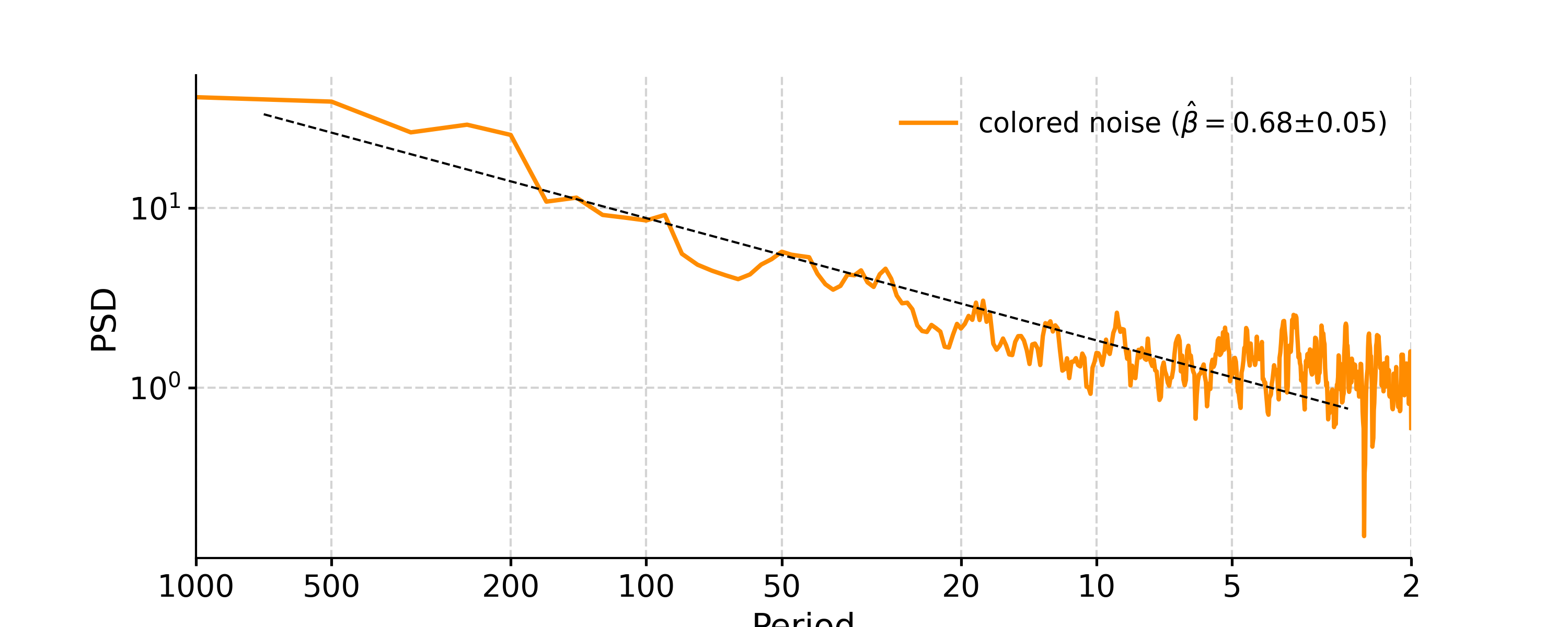
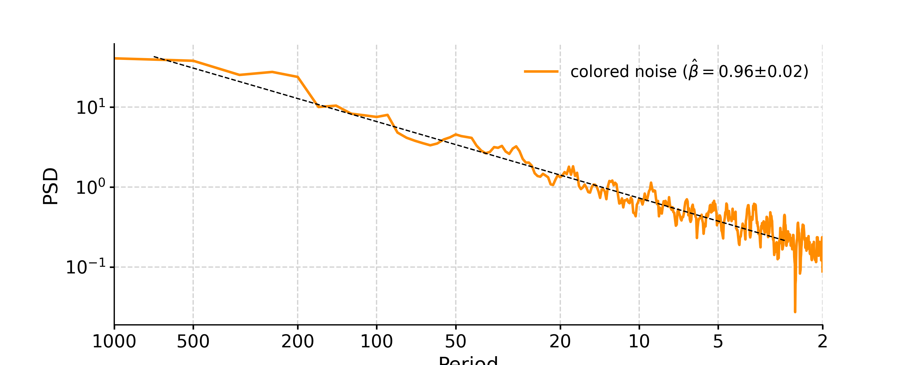
../_images/color_noise_no_anti_alias.png

References

Kirchner, J. W. Aliasing in 1/f(alpha) noise spectra: origins, consequences, and remedies. Phys Rev E Stat Nonlin Soft Matter Phys 71, 66110 (2005).

See also

pyleoclim.utils.wavelet.AliasFilter.alias_filter: anti-aliasing filter

beta_est(fmin=None, fmax=None, logf_binning_step='max', verbose=False)[source]

Estimate the scaling exponent (beta) of the PSD

For a power law S(f) ~ f^beta in log-log space, beta is simply the slope.

Parameters:

fmin (float, optional) – the minimum frequency edge for beta estimation; the default is the minimum of the frequency vector of the PSD obj
fmax (float, optional) – the maximum frequency edge for beta estimation; the default is the maximum of the frequency vector of the PSD obj
logf_binning_step (str, {'max', 'first'}) – if ‘max’, then the maximum spacing of log(f) will be used as the binning step if ‘first’, then the 1st spacing of log(f) will be used as the binning step
verbose (bool; {True, False}) – If True, will print warning messages if there is any

Returns:

new – New PSD object with the estimated scaling slope information, which is stored as a dictionary that includes: - beta: the scaling factor - std_err: the one standard deviation error of the scaling factor - f_binned: the binned frequency series, used as X for linear regression - psd_binned: the binned PSD series, used as Y for linear regression - Y_reg: the predicted Y from linear regression, used with f_binned for the slope curve plotting

Return type:

pyleoclim.core.psds.PSD

Examples

Generate fractal noise and verify that its scaling exponent is close to unity

In [1]: import pyleoclim as pyleo

In [2]: t, v = pyleo.utils.tsmodel.gen_ts(model='colored_noise')

In [3]: ts = pyleo.Series(time=t, value= v, label = 'fractal noise, unit slope')

In [4]: psd = ts.detrend().spectral(method='cwt')

# estimate the scaling slope
In [5]: psd_beta = psd.beta_est(fmin=1/50, fmax=1/2)

In [6]: fig, ax = psd_beta.plot(color='tab:blue',beta_kwargs={'color':'tab:red','linewidth':2})

In [7]: pyleo.closefig(fig)

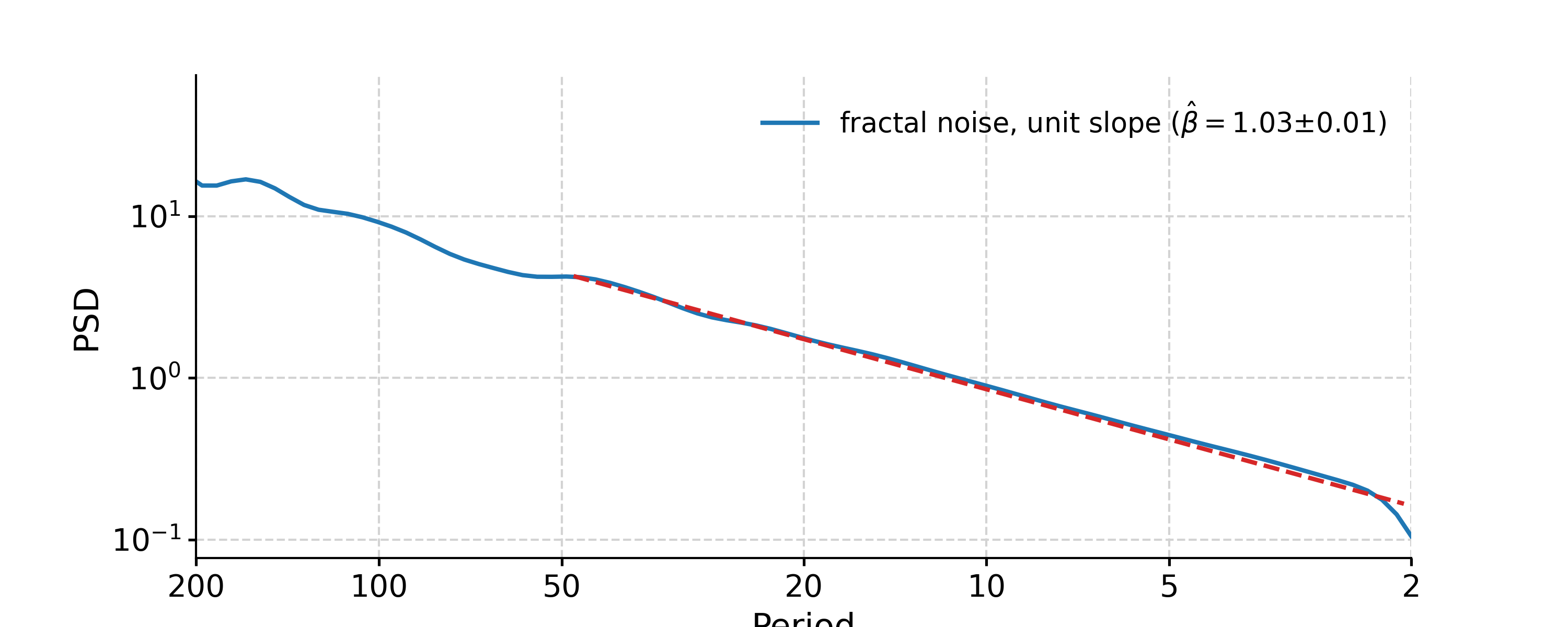
See also

pyleoclim.core.series.Series.spectral: spectral analysis
pyleoclim.utils.spectral.beta_estimation: Estimate the scaling exponent of a power spectral density
pyleoclim.core.psds.PSD.plot: plotting method for PSD objects

copy()[source]: Copy object

plot(in_loglog=True, in_period=True, label=None, xlabel=None, ylabel='PSD', title=None, marker=None, markersize=None, color=None, linestyle=None, linewidth=None, transpose=False, xlim=None, ylim=None, figsize=[10, 4], savefig_settings=None, ax=None, legend=True, lgd_kwargs=None, xticks=None, yticks=None, alpha=None, zorder=None, plot_kwargs=None, signif_clr='red', signif_linestyles=['--', '-.', ':'], signif_linewidth=1, plot_beta=True, beta_kwargs=None)[source]

Plots the PSD estimates and signif level if included

Parameters:

in_loglog (bool; {True, False}, optional) – Plot on loglog axis. The default is True.
in_period (bool; {True, False}, optional) – Plot the x-axis as periodicity rather than frequency. The default is True.
label (str, optional) – label for the series. The default is None.
xlabel (str, optional) – Label for the x-axis. The default is None. Will guess based on Series
ylabel (str, optional) – Label for the y-axis. The default is ‘PSD’.
title (str, optional) – Plot title. The default is None.
marker (str, optional) – marker to use. The default is None.
markersize (int, optional) – size of the marker. The default is None.
color (str, optional) – Line color. The default is None.
linestyle (str, optional) – linestyle. The default is None.
linewidth (float, optional) – Width of the line. The default is None.
transpose (bool; {True, False}, optional) – Plot periodicity on y-. The default is False.
xlim (list, optional) – x-axis limits. The default is None.
ylim (list, optional) – y-axis limits. The default is None.
figsize (list, optional) – Figure size. The default is [10, 4].
savefig_settings (dict, optional) –
save settings options. The default is None. the dictionary of arguments for plt.savefig(); some notes below: - “path” must be specified; it can be any existed or non-existed path,

with or without a suffix; if the suffix is not given in “path”, it will follow “format”
- ”format” can be one of {“pdf”, “eps”, “png”, “ps”}
ax (ax, optional) – The matplotlib.Axes object onto which to return the plot. The default is None.
legend (bool; {True, False}, optional) – whether to plot the legend. The default is True.
lgd_kwargs (dict, optional) – Arguments for the legend. The default is None.
xticks (list, optional) – xticks to use. The default is None.
yticks (list, optional) – yticks to use. The default is None.
alpha (float, optional) – Transparency setting. The default is None.
zorder (int, optional) – Order for the plot. The default is None.
plot_kwargs (dict, optional) – Other plotting argument. The default is None.
signif_clr (str, optional) – Color for the significance line. The default is ‘red’.
signif_linestyles (list of str, optional) – Linestyles for significance. The default is [’–’, ‘-.’, ‘:’].
signif_linewidth (float, optional) – width of the significance line. The default is 1.
plot_beta (bool; {True, False}, optional) – If True and self.beta_est_res is not None, then the scaling slope line will be plotted
beta_kwargs (dict, optional) – The visualization keyword arguments for the scaling slope

Return type:

fig, ax

Examples

Generate fractal noise, assess significance against an AR(1) benchmark, and plot:

In [1]: import matplotlib.pyplot as plt

In [2]: t, v = pyleo.utils.tsmodel.gen_ts(model='colored_noise')

In [3]: ts = pyleo.Series(time = t, value = v, label = 'fractal noise')

In [4]: tsn = ts.standardize()

In [5]: psd_sim = tsn.spectral(method='mtm').signif_test(number=20)

In [6]: psd_sim.plot()
Out[6]: 
(<Figure size 1000x400 with 1 Axes>,
 <AxesSubplot: xlabel='Period', ylabel='PSD'>)

In [7]: pyleo.closefig(fig)

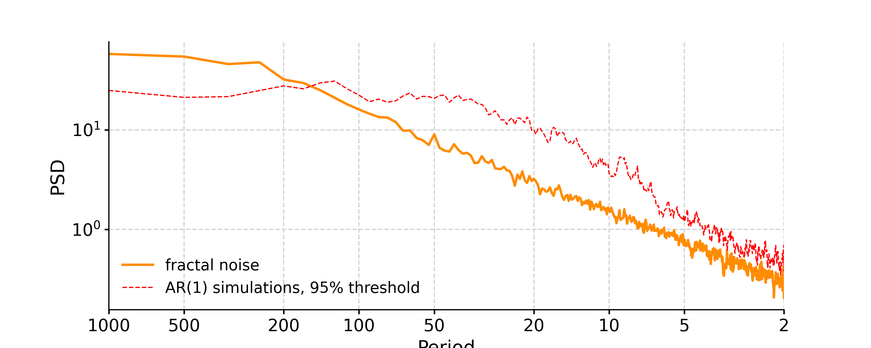
If you add the estimate of the scaling exponent, the line of best fit will be added to the plot, and the estimated exponent to its legend. For instance:

In [8]: psd_beta = psd_sim.beta_est(fmin=1/100, fmax=1/2)

In [9]: fig, ax = psd_beta.plot()

In [10]: pyleo.closefig(fig)

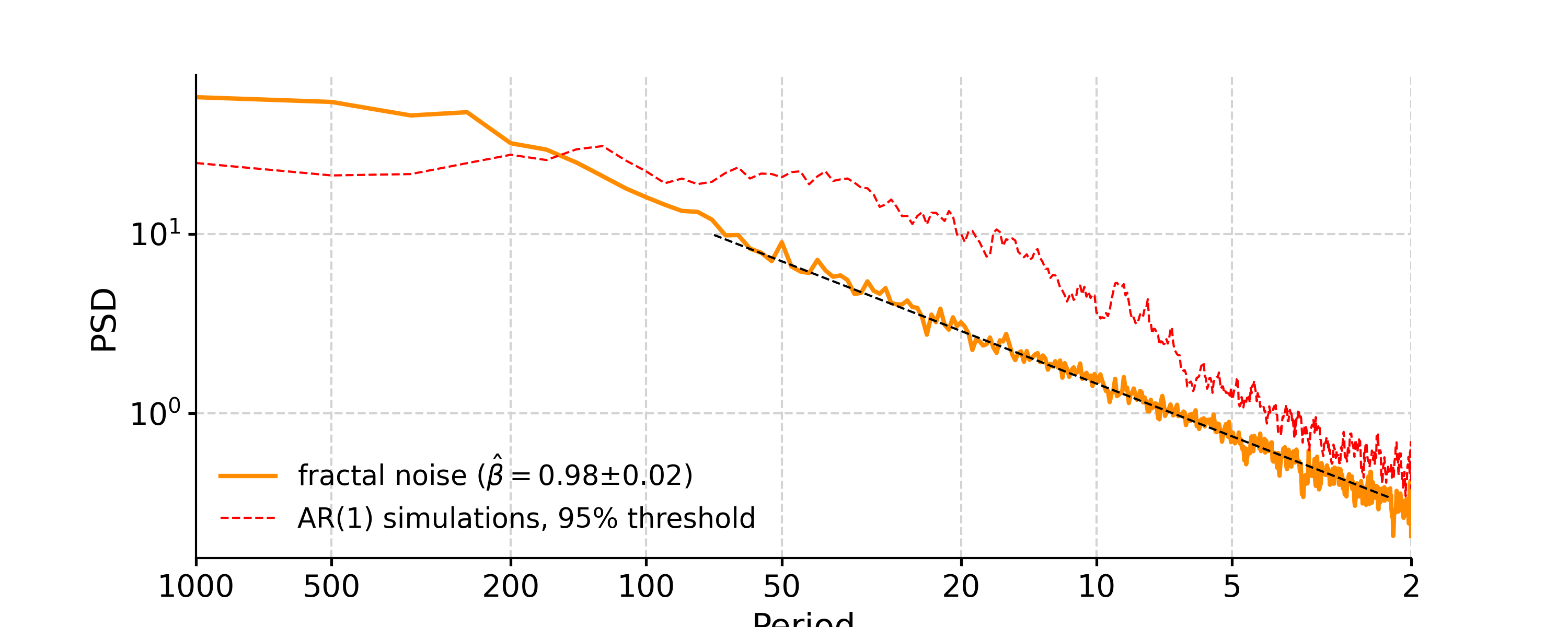
See also

pyleoclim.core.series.Series.spectral: spectral analysis
pyleoclim.core.psds.PSD.signif_test: significance testing for PSD objects
pyleoclim.core.psds.PSD.beta_est: scaling exponent estimation for PSD objects

signif_test(method='ar1sim', number=None, seed=None, qs=[0.95], settings=None, scalogram=None)[source]

Parameters:

number (int, optional) – Number of surrogate series to generate for significance testing. The default is None.
method (str; {'ar1asym','ar1sim'}) – Method to generate surrogates. AR1sim uses simulated timeseries with similar persistence. AR1asymp represents the closed form solution. The default is AR1sim
seed (int, optional) – Option to set the seed for reproducibility. The default is None.
qs (list, optional) – Significance levels to return. The default is [0.95].
settings (dict, optional) – Parameters for the specific significance test. The default is None. Note that the default value for the asymptotic solution is time-average
scalogram (pyleoclim.Scalogram object, optional) – Scalogram containing signif_scals exported during significance testing of scalogram. If number is None and signif_scals are present, will use length of scalogram list as number of significance tests

Returns:

new – New PSD object with appropriate significance test

Return type:

pyleoclim.core.psds.PSD

Examples

Compute the spectrum of the Southern Oscillation Index and assess significance against an AR(1) benchmark:

In [1]: import pandas as pd

In [2]: csv = pd.read_csv('https://raw.githubusercontent.com/LinkedEarth/Pyleoclim_util/master/example_data/soi_data.csv',skiprows = 1)

In [3]: soi = pyleo.Series(time = csv['Year'],value = csv['Value'], time_name = 'Years', time_unit = 'AD')

In [4]: psd = soi.standardize().spectral('mtm',settings={'NW':2})

In [5]: psd_sim = psd.signif_test(number=20)

In [6]: fig, ax = psd_sim.plot()

In [7]: pyleo.closefig(fig)

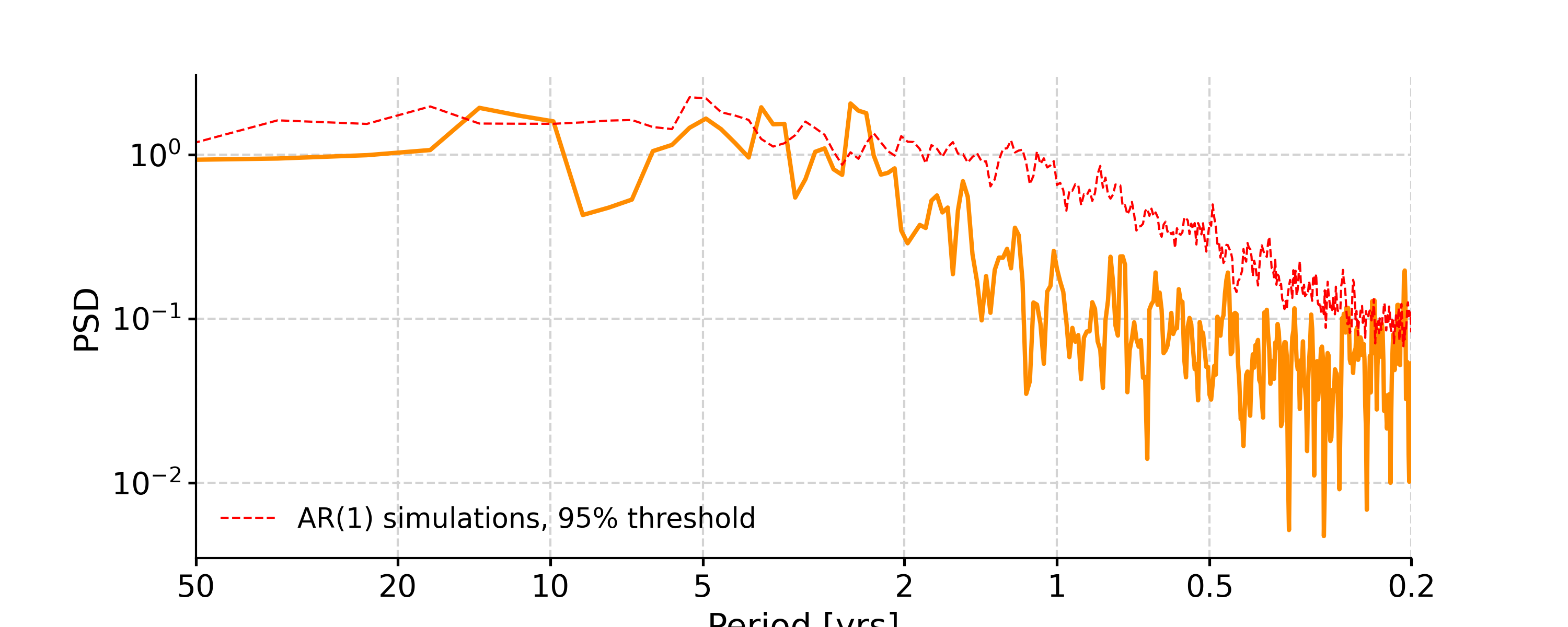
By default, this method uses 200 Monte Carlo simulations of an AR(1) process. For a smoother benchmark, up the number of simulations. Also, you may obtain and visualize several quantiles at once, e.g. 90% and 95%:

In [8]: psd_1000 = psd.signif_test(number=100, qs=[0.90, 0.95])

In [9]: fig, ax = psd_1000.plot()

In [10]: pyleo.closefig(fig)

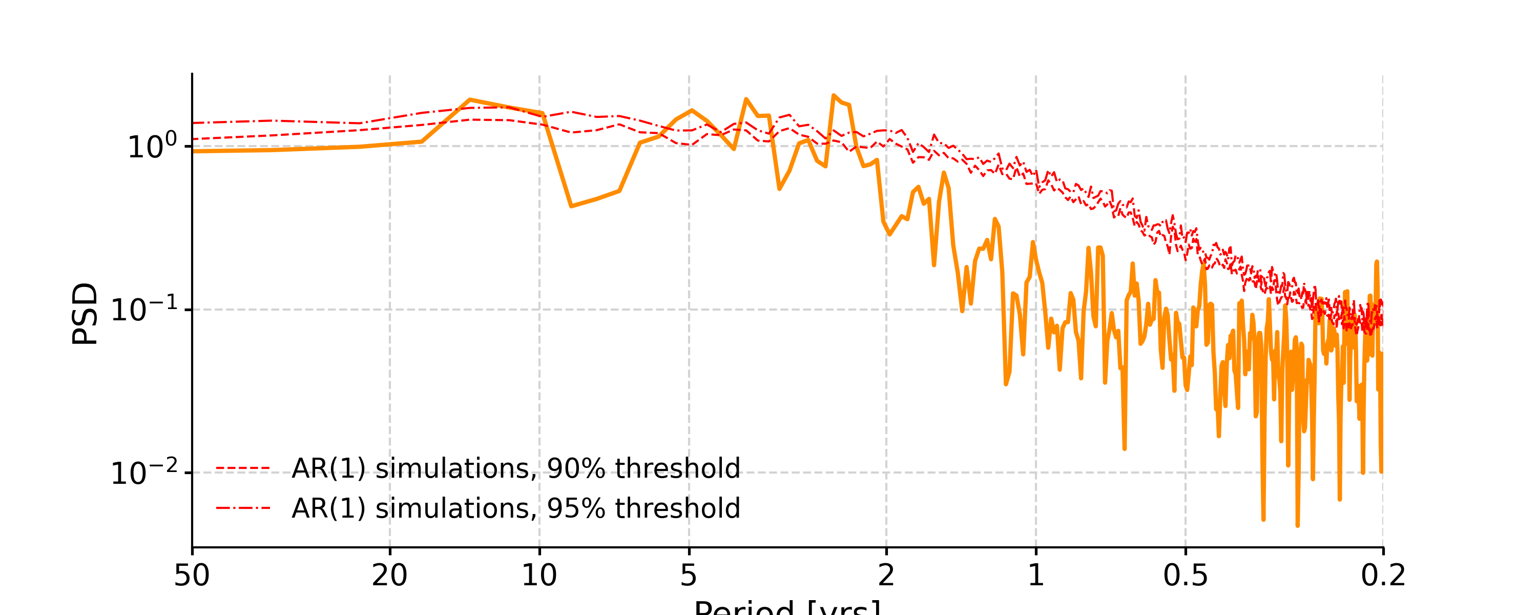
Another option is to use a closed-form, asymptotic solution for the AR(1) spectrum:

In [11]: psd_asym = psd.signif_test(method='ar1asym',qs=[0.90, 0.95])

In [12]: fig, ax = psd_asym.plot()

In [13]: pyleo.closefig(fig)

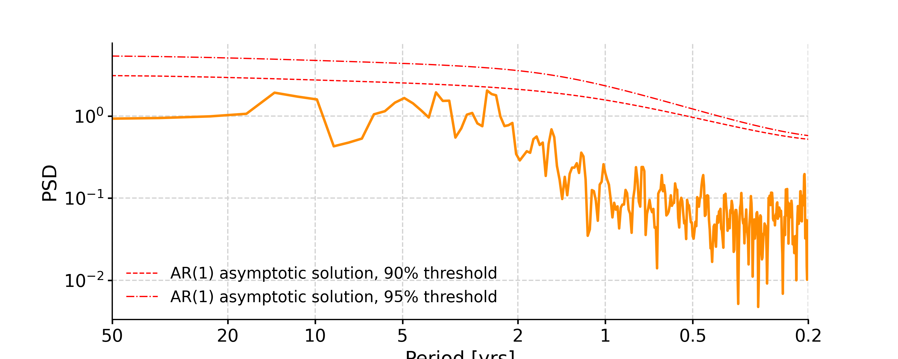
If significance tests from a comparable scalogram have been saved, they can be passed here to speed up the generation of noise realizations for significance testing. Setting export_scal to True saves the noise realizations generated during significance testing for future use:

In [14]: scalogram = soi.standardize().wavelet().signif_test(number=20, export_scal=True)

The psd can be calculated by using the previously generated scalogram

In [15]: psd_scal = soi.standardize().spectral(scalogram=scalogram)

The same scalogram can then be passed to do significance testing. Pyleoclim will dig through the scalogram object to find the saved noise realizations and reuse them flexibly.

In [16]: fig, ax = psd.signif_test(scalogram=scalogram).plot()

In [17]: pyleo.closefig(fig)

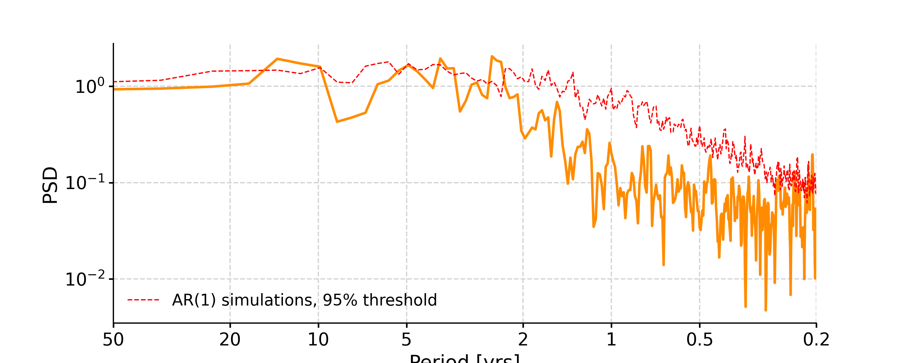
See also

pyleoclim.utils.wavelet.tc_wave_signif: asymptotic significance calculation
pyleoclim.core.psds.MultiplePSD: Object storing several PSDs from different Series or ensemble members in an age model
pyleoclim.core.scalograms.Scalogram: Scalogram object
pyleoclim.core.series.Series.surrogates: Generate surrogates with increasing time axis
pyleoclim.core.series.Series.spectral: Performs spectral analysis on Pyleoclim Series
pyleoclim.core.series.Series.wavelet: Performs wavelet analysis on Pyleoclim Series

MultiplePSD (pyleoclim.MultiplePSD)

class pyleoclim.core.psds.MultiplePSD(psd_list, beta_est_res=None)[source]
MultiplePSD objects store several PSDs from different Series or ensemble members from a posterior distribution (e.g. age model, Bayesian climate reconstruction, etc). This is used extensively for Monte Carlo significance tests.

Methods

anti_alias([avgs, mute_pbar])

Apply the anti-aliasing filter

beta_est([fmin, fmax, logf_binning_step, ...])

Estimate the scaling exponent of each constituent PSD

copy()

Copy object

plot([figsize, in_loglog, in_period, ...])

Plot multiple PSDs on the same plot

plot_envelope([figsize, qs, in_loglog, ...])

Plot an envelope statistics for mulitple PSD

quantiles([qs, lw])

Calculate the quantiles of the significance testing

anti_alias(avgs=2, mute_pbar=False)[source]

Apply the anti-aliasing filter

Parameters:

avgs (int) – flag for whether spectrum is derived from instantaneous point measurements (avgs<>1) OR from measurements averaged over each sampling interval (avgs==1)

mute_pbar (bool; {True,False}) – If True, the progressbar will be muted. Default is False.

Returns:

new – New MultiplePSD object with the spectral aliasing effect alleviated.

Return type:

pyleoclim.core.psds.MultiplePSD

References

Kirchner, J. W. Aliasing in 1/f(alpha) noise spectra: origins, consequences, and remedies. Phys Rev E Stat Nonlin Soft Matter Phys 71, 66110 (2005).

See also

pyleoclim.utils.wavelet.AliasFilter.alias_filter
anti-aliasing filter

beta_est(fmin=None, fmax=None, logf_binning_step='max', verbose=False)[source]

Estimate the scaling exponent of each constituent PSD

This function calculates the scaling exponent (beta) for each of the PSDs stored in the object. The scaling exponent represents the slope of the spectrum in log-log space.

Parameters:

fmin (float) – the minimum frequency edge for beta estimation; the default is the minimum of the frequency vector of the PSD object

fmax (float) – the maximum frequency edge for beta estimation; the default is the maximum of the frequency vector of the PSD object

logf_binning_step (str; {'max', 'first'}) – if ‘max’, then the maximum spacing of log(f) will be used as the binning step. if ‘first’, then the 1st spacing of log(f) will be used as the binning step.

verbose (bool) – If True, will print warning messages if there is any

Returns:

new – New MultiplePSD object with the estimated scaling slope information, which is stored as a dictionary that includes: - beta: the scaling factor - std_err: the one standard deviation error of the scaling factor - f_binned: the binned frequency series, used as X for linear regression - psd_binned: the binned PSD series, used as Y for linear regression - Y_reg: the predicted Y from linear regression, used with f_binned for the slope curve plotting

Return type:

pyleoclim.core.psds.MultiplePSD

See also

pyleoclim.core.psds.PSD.beta_est
scaling exponent estimation for a single PSD object

copy()[source]

Copy object

plot(figsize=[10, 4], in_loglog=True, in_period=True, xlabel=None, ylabel='PSD', title=None, xlim=None, ylim=None, savefig_settings=None, ax=None, xticks=None, yticks=None, legend=True, colors=None, cmap=None, norm=None, plot_kwargs=None, lgd_kwargs=None)[source]

Plot multiple PSDs on the same plot

Parameters:

figsize (list, optional) – Figure size. The default is [10, 4].

in_loglog (bool, optional) – Whether to plot in loglog. The default is True.

in_period (bool, {True, False} optional) – Plots against periods instead of frequencies. The default is True.

xlabel (str, optional) – x-axis label. The default is None.

ylabel (str, optional) – y-axis label. The default is ‘Amplitude’.

title (str, optional) – Title for the figure. The default is None.

xlim (list, optional) – Limits for the x-axis. The default is None.

ylim (list, optional) – limits for the y-axis. The default is None.

colors (a list of, or one, Python supported color code (a string of hex code or a tuple of rgba values)) – Colors for plotting. If None, the plotting will cycle the ‘tab10’ colormap; if only one color is specified, then all curves will be plotted with that single color; if a list of colors are specified, then the plotting will cycle that color list.

cmap (str) – The colormap to use when “colors” is None.

norm (matplotlib.colors.Normalize like) – The nomorlization for the colormap. If None, a linear normalization will be used.

savefig_settings (dict, optional) –
the dictionary of arguments for plt.savefig(); some notes below: - “path” must be specified; it can be any existing or non-existing path,

with or without a suffix; if the suffix is not given in “path”, it will follow “format”

”format” can be one of {“pdf”, “eps”, “png”, “ps”}

ax (matplotlib axis, optional) – The matplotlib axis object on which to retrun the figure. The default is None.

xticks (list, optional) – x-ticks label. The default is None.

yticks (list, optional) – y-ticks label. The default is None.

legend (bool, optional) – Whether to plot the legend. The default is True.

plot_kwargs (dictionary, optional) – Parameters for plot function. The default is None.

lgd_kwargs (dictionary, optional) – Parameters for legend. The default is None.

Returns:

fig (matplotlib.pyplot.figure)

ax (matplotlib.pyplot.axis)

See also

pyleoclim.core.psds.PSD.plot
plotting method for PSD objects
plot_envelope(figsize=[10, 4], qs=[0.025, 0.5, 0.975], in_loglog=True, in_period=True, xlabel=None, ylabel='PSD', title=None, xlim=None, ylim=None, savefig_settings=None, ax=None, xticks=None, yticks=None, plot_legend=True, curve_clr='#d9544d', curve_lw=3, shade_clr='#d9544d', shade_alpha=0.3, shade_label=None, lgd_kwargs=None, members_plot_num=10, members_alpha=0.3, members_lw=1, seed=None)[source]
Plot an envelope statistics for mulitple PSD

This function plots an envelope statistics from multiple PSD. This is especially useful when the PSD are coming from an ensemble of possible solutions (e.g., age ensembles)

Parameters:

figsize (list, optional) – The figure size. The default is [10, 4].

qs (list, optional) – The significance levels to consider. The default is [0.025, 0.5, 0.975].

in_loglog (bool, optional) – Plot in log space. The default is True.

in_period (bool, optional) – Whether to plot periodicity instead of frequency. The default is True.

xlabel (str, optional) – x-axis label. The default is None.

ylabel (str, optional) – y-axis label. The default is ‘Amplitude’.

title (str, optional) – Plot title. The default is None.

xlim (list, optional) – x-axis limits. The default is None.

ylim (list, optional) – y-axis limits. The default is None.

savefig_settings (dict, optional) –
the dictionary of arguments for plt.savefig(); some notes below: - “path” must be specified; it can be any existing or non-existing path,

with or without a suffix; if the suffix is not given in “path”, it will follow “format”

”format” can be one of {“pdf”, “eps”, “png”, “ps”} The default is None.

ax (matplotlib.ax, optional) – Matplotlib axis on which to return the plot. The default is None.

xticks (list, optional) – xticks label. The default is None.

yticks (list, optional) – yticks label. The default is None.

plot_legend (bool, optional) – Wether to plot the legend. The default is True.

curve_clr (str, optional) – Color of the main PSD. The default is sns.xkcd_rgb[‘pale red’].

curve_lw (str, optional) – Width of the main PSD line. The default is 3.

shade_clr (str, optional) – Color of the shaded envelope. The default is sns.xkcd_rgb[‘pale red’].

shade_alpha (float, optional) – Transparency on the envelope. The default is 0.3.

shade_label (str, optional) – Label for the envelope. The default is None.

lgd_kwargs (dict, optional) – Parameters for the legend. The default is None.

members_plot_num (int, optional) – Number of individual members to plot. The default is 10.

members_alpha (float, optional) – Transparency of the lines representing the multiple members. The default is 0.3.

members_lw (float, optional) – With of the lines representing the multiple members. The default is 1.

seed (int, optional) – Set the seed for random number generator. Useful for reproducibility. The default is None.

Returns:

fig (matplotlib.pyplot.figure)

ax (matplotlib.pyplot.axis)

See also

pyleoclim.core.psds.PSD.plot
plotting method for PSD objects

pyleoclim.core.ensembleseries.EnsembleSeries.plot_envelope
envelope plot for ensembles

Examples
In [1]: import pyleoclim as pyleo

In [2]: import numpy as np

In [3]: nn = 30 # number of noise realizations

In [4]: nt = 500 # timeseries length

In [5]: psds = []

In [6]: time, signal = pyleo.utils.gen_ts(model='colored_noise',nt=nt,alpha=1.0)

In [7]: ts = pyleo.Series(time=time, value = signal).standardize()

In [8]: noise = np.random.randn(nt,nn)

In [9]: for idx in range(nn):  # noise
   ...:     ts = pyleo.Series(time=time, value=signal+10*noise[:,idx])
   ...:     psd = ts.spectral()
   ...:     psds.append(psd)
   ...: 

In [10]: mPSD = pyleo.MultiplePSD(psds)

In [11]: fig, ax = mPSD.plot_envelope()

In [12]: pyleo.closefig(fig)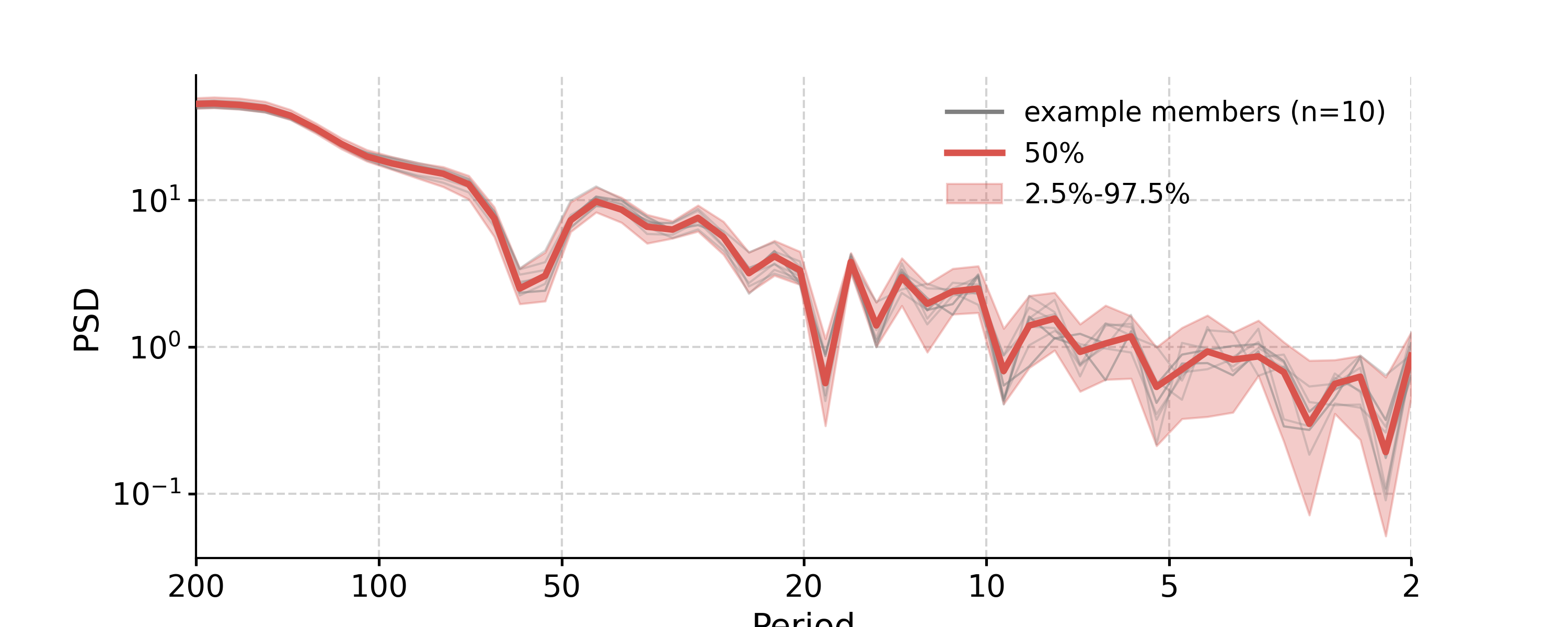
quantiles(qs=[0.05, 0.5, 0.95], lw=[0.5, 1.5, 0.5])[source]

Calculate the quantiles of the significance testing

Parameters:

qs (list, optional) – List of quantiles to consider for the calculation. The default is [0.05, 0.5, 0.95].

lw (list, optional) – Linewidth to use for plotting each level. Should be the same length as qs. The default is [0.5, 1.5, 0.5].

Raises:

ValueError – Frequency axis not consistent across the PSD list!

Returns:

psds

Return type:

pyleoclim.core.psds.MultiplePSD

Scalogram (pyleoclim.Scalogram)

class pyleoclim.core.scalograms.Scalogram(frequency, scale, time, amplitude, coi=None, label=None, Neff_threshold=3, wwz_Neffs=None, timeseries=None, wave_method=None, wave_args=None, signif_qs=None, signif_method=None, freq_method=None, freq_kwargs=None, scale_unit=None, time_label=None, signif_scals=None, qs=None)[source]

The Scalogram class is analogous to PSD, but for wavelet spectra (scalograms).

Methods

`copy`()	Copy object
`plot`([variable, in_scale, xlabel, ylabel, ...])	Plot the scalogram
`signif_test`([method, number, seed, qs, ...])	Significance test for scalograms

copy()[source]

Copy object

Returns:: scal – The copied version of the pyleoclim.Scalogram object
Return type:: pyleoclim.core.scalograms.Scalogram

Examples

In [1]: import pyleoclim as pyleo

In [2]: import pandas as pd

In [3]: ts=pd.read_csv('https://raw.githubusercontent.com/LinkedEarth/Pyleoclim_util/master/example_data/soi_data.csv',skiprows = 1)

In [4]: series = pyleo.Series(time = ts['Year'],value = ts['Value'], time_name = 'Years', time_unit = 'AD')

In [5]: scalogram = series.wavelet()

In [6]: scalogram_copy = scalogram.copy()

plot(variable='amplitude', in_scale=True, xlabel=None, ylabel=None, title=None, ylim=None, xlim=None, yticks=None, figsize=[10, 8], signif_clr='white', signif_linestyles='-', signif_linewidths=1, contourf_style={}, cbar_style={}, plot_cb=True, savefig_settings={}, ax=None, signif_thresh=0.95)[source]

Plot the scalogram

Parameters:

in_scale (bool, optional) – Plot the in scale instead of frequency space. The default is True.
variable ({'amplitude','power'}) – Whether to plot the amplitude or power. Default is amplitude
xlabel (str, optional) – Label for the x-axis. The default is None.
ylabel (str, optional) – Label for the y-axis. The default is None.
title (str, optional) – Title for the figure. The default is ‘default’, which auto-generates a title.
ylim (list, optional) – Limits for the y-axis. The default is None.
xlim (list, optional) – Limits for the x-axis. The default is None.
yticks (list, optional) – yticks label. The default is None.
figsize (list, optional) – Figure size The default is [10, 8].
signif_clr (str, optional) – Color of the singificance line. The default is ‘white’.
signif_thresh (float in [0, 1]) – Significance threshold. Default is 0.95. If this quantile is not found in the qs field of the Coherence object, the closest quantile will be picked.
signif_linestyles (str, optional) – Linestyle of the significance line. The default is ‘-‘.
signif_linewidths (float, optional) – Width for the significance line. The default is 1.
contourf_style (dict, optional) – Arguments for the contour plot. The default is {}.
cbar_style (dict, optional) – Arguments for the colarbar. The default is {}.
savefig_settings (dict, optional) – saving options for the figure. The default is {}.
ax (ax, optional) – Matplotlib Axis on which to return the figure. The default is None.

Returns:

fig (matplotlib.figure) – the figure object from matplotlib See [matplotlib.pyplot.figure](https://matplotlib.org/3.1.1/api/_as_gen/matplotlib.pyplot.figure.html) for details.
ax (matplotlib.axis) – the axis object from matplotlib See [matplotlib.axes](https://matplotlib.org/api/axes_api.html) for details.

See also

pyleoclim.core.series.Series.wavelet: Wavelet analysis
pyleoclim.utils.plotting.savefig: Saving figure in Pyleoclim

Examples

In [1]: import pyleoclim as pyleo

In [2]: import pandas as pd

In [3]: ts=pd.read_csv('https://raw.githubusercontent.com/LinkedEarth/Pyleoclim_util/master/example_data/soi_data.csv',skiprows = 1)

In [4]: series = pyleo.Series(time = ts['Year'],value = ts['Value'], time_name = 'Years', time_unit = 'AD')

In [5]: scalogram = series.wavelet()

In [6]: fig,ax = scalogram.plot()

In [7]: pyleo.closefig(fig)

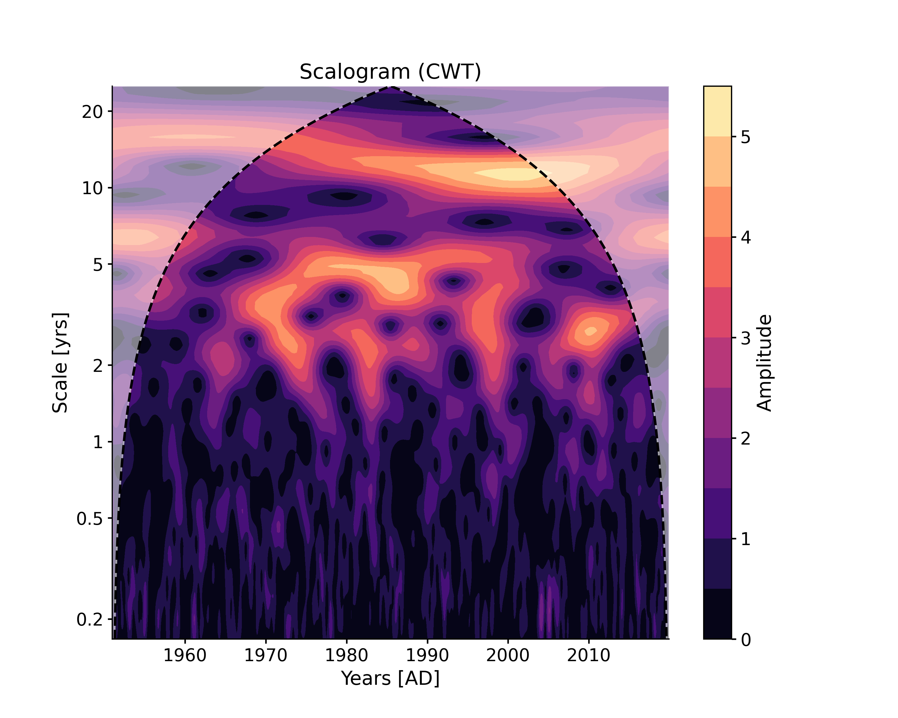
signif_test(method='ar1sim', number=None, seed=None, qs=[0.95], settings=None, export_scal=False)[source]

Significance test for scalograms

Parameters:

method{‘ar1asym’, ‘ar1sim’}

Method to use to generate the surrogates. ar1sim uses simulated timeseries with similar persistence. ar1asym represents the theoretical, closed-form solution. The default is ar1sim

numberint

Number of surrogates to generate for significance analysis based on simulations. The default is 200.

seed : int, optional

Set the seed for the random number generator. Useful for reproducibility The default is None.

qs : list, optional

Significane level to consider. The default is [0.95].

settings : dict, optional

Parameters for the model. The default is None.

export_scal : bool; {True,False}

Whether or not to export the scalograms used in the noise realizations. Note: For the wwz method, the scalograms used for wavelet analysis are slightly different than those used for spectral analysis (different decay constant). As such, this functionality should be used only to expedite exploratory analysis.

Returns:

newpyleoclim.core.scalograms.Scalogram: A new Scalogram object with the significance level

Raises:

ValueError: qs should be a list with at least one value.

See also

pyleoclim.core.series.Series.wavelet: Wavelet analysis
pyleoclim.core.scalograms.MultipleScalogram: MultipleScalogram object
pyleoclim.utils.wavelet.tc_wave_signif: Asymptotic significance calculation

Examples

Generating scalogram, running significance tests, and saving the output for future use in generating psd objects or in summary_plot()

In [1]: import pyleoclim as pyleo

In [2]: import pandas as pd

In [3]: ts=pd.read_csv('https://raw.githubusercontent.com/LinkedEarth/Pyleoclim_util/master/example_data/soi_data.csv',skiprows = 1)

In [4]: series = pyleo.Series(time = ts['Year'],value = ts['Value'], time_name = 'Years', time_unit = 'AD')

By setting export_scal to True, the noise realizations used to generate the significance test will be saved. These come in handy for generating summary plots and for running significance tests on spectral objects.

In [5]: scalogram = series.wavelet().signif_test(number=2, export_scal=True)

MultipleScalogram (pyleoclim.MultipleScalogram)

class pyleoclim.core.scalograms.MultipleScalogram(scalogram_list)[source]

MultipleScalogram objects are used to store the results of significance testing for wavelet analysis

Methods

`copy`()	Copy the object
`quantiles`([qs])	Calculate quantiles

copy()[source]

Copy the object

See also

pyleoclim.core.scalograms.Scalogram.copy: Scalogram object copy

quantiles(qs=[0.05, 0.5, 0.95])[source]

Calculate quantiles

Parameters:

qs (list, optional) – List of quantiles to consider for the calculation. The default is [0.05, 0.5, 0.95].

Raises:

ValueError – Frequency axis not consistent across the PSD list!
Value Error – Time axis not consistent across the scalogram list!

Returns:

scals

Return type:

pyleoclim.core.scalograms.MultipleScalogram

Coherence (pyleoclim.Coherence)

class pyleoclim.core.coherence.Coherence(frequency, scale, time, wtc, xwt, phase, coi=None, wave_method=None, wave_args=None, timeseries1=None, timeseries2=None, signif_qs=None, signif_method=None, qs=None, freq_method=None, freq_kwargs=None, Neff_threshold=3, scale_unit=None, time_label=None)[source]

Coherence object, meant to receive the WTC and XWT part of Series.wavelet_coherence()

See also

pyleoclim.core.series.Series.wavelet_coherence: Wavelet coherence method

Methods

`copy`()	Copy object
`dashboard`([title, figsize, phase_style, ...])	Cross-wavelet dashboard, including the two series, WTC and XWT.
`phase_stats`(scales[, number, level])	Estimate phase angle statistics of a Coherence object
`plot`([var, xlabel, ylabel, title, figsize, ...])	Plot the cross-wavelet results
`signif_test`([number, method, seed, qs, ...])	Significance testing for Coherence objects

copy()[source]: Copy object

dashboard(title=None, figsize=[9, 12], phase_style={}, line_colors=['tab:blue', 'tab:orange'], savefig_settings={}, ts_plot_kwargs=None, wavelet_plot_kwargs=None)[source]

Cross-wavelet dashboard, including the two series, WTC and XWT.

Note: this design balances many considerations, and is not easily customizable.

Parameters:

title (str, optional) – Title of the plot. The default is None.
figsize (list, optional) – Figure size. The default is [9, 12], as this is an information-rich figure.
line_colors (list, optional) – Colors for the 2 traces For nomenclature, see https://matplotlib.org/stable/gallery/color/named_colors.html
savefig_settings (dict, optional) –
The default is {}. the dictionary of arguments for plt.savefig(); some notes below: - “path” must be specified; it can be any existed or non-existed path,

with or without a suffix; if the suffix is not given in “path”, it will follow “format”
- ”format” can be one of {“pdf”, “eps”, “png”, “ps”}
phase_style (dict, optional) – Arguments for the phase arrows. The default is {}. It includes: - ‘pt’: the default threshold above which phase arrows will be plotted - ‘skip_x’: the number of points to skip between phase arrows along the x-axis - ‘skip_y’: the number of points to skip between phase arrows along the y-axis - ‘scale’: number of data units per arrow length unit (see matplotlib.pyplot.quiver) - ‘width’: shaft width in arrow units (see matplotlib.pyplot.quiver) - ‘color’: arrow color (see matplotlib.pyplot.quiver)
ts_plot_kwargs (dict) – arguments to be passed to the timeseries subplot, see pyleoclim.core.series.Series.plot for details
wavelet_plot_kwargs (dict) – arguments to be passed to the contour subplots (XWT and WTC), [see pyleoclim.core.coherence.Coherence.plot for details]

Return type:

fig, ax

See also

pyleoclim.core.coherence.Coherence.plot: creates a coherence plot
pyleoclim.core.series.Series.wavelet_coherence: computes the coherence between two timeseries.
pyleoclim.core.series.Series.plot: plots a timeseries
matplotlib.pyplot.quiver: makes a quiver plot

Examples

Calculate the coherence of NINO3 and All India Rainfall and plot it as a dashboard:

In [1]: import pyleoclim as pyleo

In [2]: import pandas as pd

In [3]: data = pd.read_csv('https://raw.githubusercontent.com/LinkedEarth/Pyleoclim_util/Development/example_data/wtc_test_data_nino_even.csv')

In [4]: time = data['t'].values

In [5]: ts_air = pyleo.Series(time=time, value=data['air'].values, time_name='Year (CE)',
   ...:                       label='All India Rainfall', value_name='AIR (mm/month)')
   ...: 

In [6]: ts_nino = pyleo.Series(time=time, value=data['nino'].values, time_name='Year (CE)',
   ...:                        label='NINO3', value_name='NINO3 (K)')
   ...: 

In [7]: coh = ts_air.wavelet_coherence(ts_nino)

In [8]: coh_sig = coh.signif_test(number=10)

In [9]: coh_sig.dashboard()
Out[9]: 
(<Figure size 900x1200 with 6 Axes>,
 {'ts1': <AxesSubplot: ylabel='AIR (mm/month)'>,
  'ts2': <AxesSubplot: xlabel='Year (CE)', ylabel='NINO3 (K)'>,
  'wtc': <AxesSubplot: ylabel='Scale'>,
  'xwt': <AxesSubplot: xlabel='Year (CE)', ylabel='Scale'>})

In [10]: pyleo.closefig(fig)

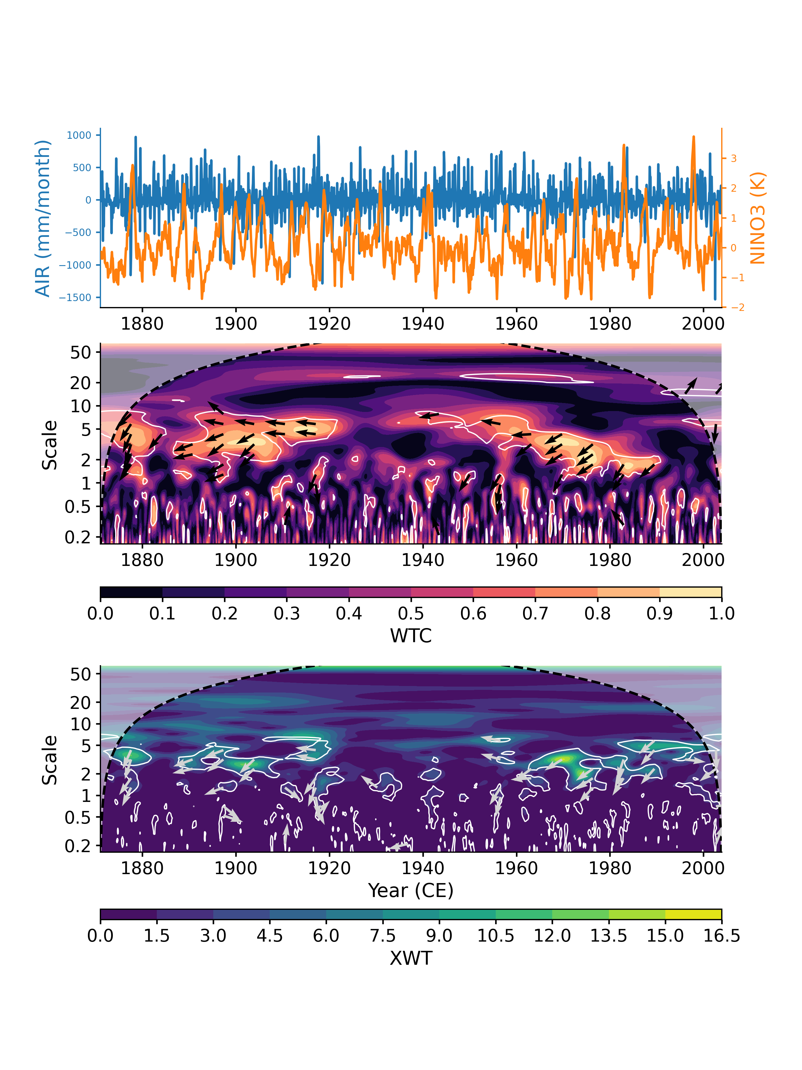
You may customize colors like so:

In [11]: coh_sig.dashboard(line_colors=['teal','gold'])
Out[11]: 
(<Figure size 900x1200 with 6 Axes>,
 {'ts1': <AxesSubplot: ylabel='AIR (mm/month)'>,
  'ts2': <AxesSubplot: xlabel='Year (CE)', ylabel='NINO3 (K)'>,
  'wtc': <AxesSubplot: ylabel='Scale'>,
  'xwt': <AxesSubplot: xlabel='Year (CE)', ylabel='Scale'>})

In [12]: pyleo.closefig(fig)

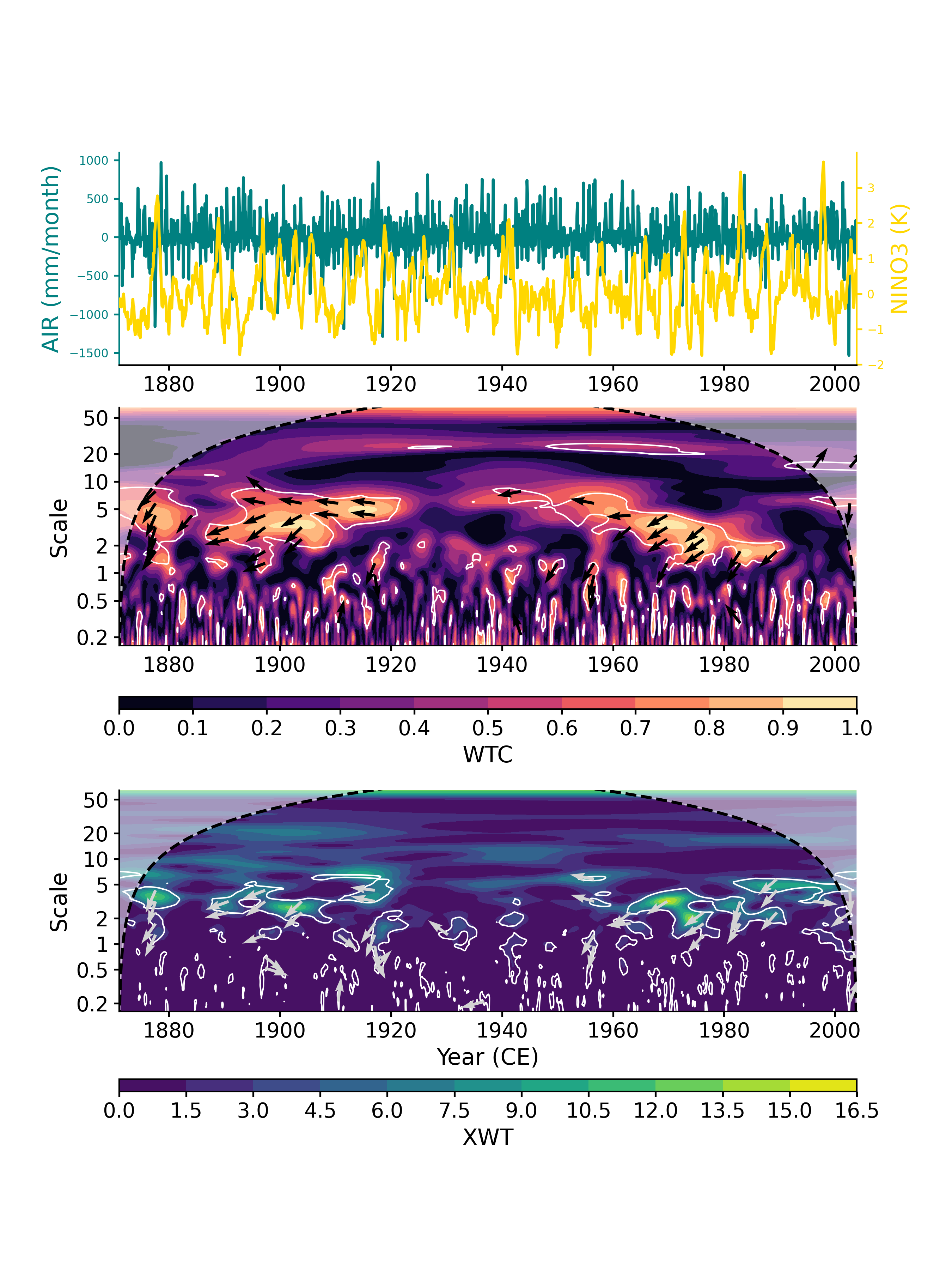
To export the figure, use savefig_settings:

In [13]: coh_sig.dashboard(savefig_settings={'path':'coh_dash.png','dpi':300})
Figure saved at: "coh_dash.png"
Out[13]: 
(<Figure size 900x1200 with 6 Axes>,
 {'ts1': <AxesSubplot: ylabel='AIR (mm/month)'>,
  'ts2': <AxesSubplot: xlabel='Year (CE)', ylabel='NINO3 (K)'>,
  'wtc': <AxesSubplot: ylabel='Scale'>,
  'xwt': <AxesSubplot: xlabel='Year (CE)', ylabel='Scale'>})

In [14]: pyleo.closefig(fig)

phase_stats(scales, number=1000, level=0.05)[source]

Estimate phase angle statistics of a Coherence object

As per [1], the strength (consistency) of a phase relationship is assessed using:

sigma, the circular standard deviation
kappa, an estimate of the Von Mises distribution’s concentration parameter.
It is a reciprocal measure of dispersion, so 1/kappa is analogous to the variance) [3].

Because of inherent persistence of geophysical signals and of the reproducing kernel of the continuous wavelet transform [3], phase statistics are assessed relative to an AR(1) model fit to the angle deviations observed at the requested scale(s).

Specifically, if number is specified, the method simulates number Monte Carlo realizations of an AR(1) process fit to fluctuations around the mean angle. This ensemble is used to obtain the confidence limits: sigma_lo (level quantile) and kappa_hi (1-level quantile). These correspond to 1-tailed tests of the strength of the relationship.

Parameters:

scales (float) – scale at which to evaluate the phase angle
number (int, optional) – number of AR(1) series to create for significance testing. The default is 1000.
level (float, optional) – significance level against which to gauge sigma and kappa. default: 0.05

Returns:

result – contains angle_mean (the mean angle for those scales), sigma (the circular standard deviation), kappa, sigma_lo (alpha-level quantile for sigma) and kappa_hi, the (1-alpha)-level quantile for kappa.

Return type:

dict

See also

pyleoclim.core.series.Series.wavelet_coherence: Wavelet coherence
pyleoclim.core.scalograms.Scalogram: Scalogram object
pyleoclim.core.scalograms.MultipleScalogram: Multiple Scalogram object
pyleoclim.core.coherence.Coherence.plot: plotting method for Coherence objects
pyleoclime.utils.wavelet.angle_sig: significance of phase angle statistics
pyleoclim.utils.wavelet.angle_stats: phase angle statistics

References

[1] Grinsted, A., J. C. Moore, and S. Jevrejeva (2004), Application of the cross wavelet transform and wavelet coherence to geophysical time series, Nonlinear Processes in Geophysics, 11, 561–566.

[2] Huber, R., Dutra, L. V., & da Costa Freitas, C. (2001). SAR interferogram phase filtering based on the Von Mises distribution. In IGARSS 2001. Scanning the Present and Resolving the Future. Proceedings. IEEE 2001 International Geoscience and Remote Sensing Symposium (Cat. No. 01CH37217) (Vol. 6, pp. 2816-2818). IEEE.

[3] Farge, M. and Schneider, K. (2006): Wavelets: application to turbulence Encyclopedia of Mathematical Physics (Eds. J.-P. Françoise, G. Naber and T.S. Tsun) pp 408-420.

Examples

Calculate the phase angle between NINO3 and All India Rainfall at 5y scales:

In [1]: import pyleoclim as pyleo

In [2]: import pandas as pd

In [3]: import numpy as np

In [4]: data = pd.read_csv('https://raw.githubusercontent.com/LinkedEarth/Pyleoclim_util/Development/example_data/wtc_test_data_nino_even.csv')

In [5]: time = data['t'].values

In [6]: air = data['air'].values

In [7]: nino = data['nino'].values

In [8]: ts_air = pyleo.Series(time=time, value=air, time_name='Year (CE)',
   ...:                       label='All India Rainfall', value_name='AIR (mm/month)')
   ...: 

In [9]: ts_nino = pyleo.Series(time=time, value=nino, time_name='Year (CE)',
   ...:                        label='NINO3', value_name='NINO3 (K)')
   ...: 

In [10]: coh = ts_air.wavelet_coherence(ts_nino)

In [11]: coh.phase_stats(scales=5)
Out[11]: Results(mean_angle=-2.681280900274463, kappa=3.501981136031572, sigma=0.5853789381725574, kappa_hi=0.636291938499562, sigma_lo=1.5450107616672135)

One may also obtain phase angle statistics over an interval, like the 2-8y ENSO band:

In [12]: phase = coh.phase_stats(scales=[2,8])

In [13]: print("The mean angle is {:4.2f}°".format(phase.mean_angle/np.pi*180))
The mean angle is -154.37°

In [14]: print(phase)
Results(mean_angle=-2.6942962667703174, kappa=3.354906855356427, sigma=0.6019130803751228, kappa_hi=0.48911209085954216, sigma_lo=1.695536468114175)

From this example, one diagnoses a strong anti-phased relationship in the ENSO band, with high von Mises concentration (kappa ~ 3.35 >> kappa_hi) and low circular dispersion (sigma ~ 0.6 << sigma_lo). This would be strong evidence of a consistent anti-phasing between NINO3 and AIR at those scales.

plot(var='wtc', xlabel=None, ylabel=None, title='auto', figsize=[10, 8], ylim=None, xlim=None, in_scale=True, yticks=None, contourf_style={}, phase_style={}, cbar_style={}, savefig_settings={}, ax=None, signif_clr='white', signif_linestyles='-', signif_linewidths=1, signif_thresh=0.95, under_clr='ivory', over_clr='black', bad_clr='dimgray')[source]

Plot the cross-wavelet results

Parameters:

var (str {'wtc', 'xwt'}) – variable to be plotted as color field. Default: ‘wtc’, the wavelet transform coherency. ‘xwt’ plots the cross-wavelet transform instead.
xlabel (str, optional) – x-axis label. The default is None.
ylabel (str, optional) – y-axis label. The default is None.
title (str, optional) – Title of the plot. The default is ‘auto’, where it is made from object metadata. To mute, pass title = None.
figsize (list, optional) – Figure size. The default is [10, 8].
ylim (list, optional) – y-axis limits. The default is None.
xlim (list, optional) – x-axis limits. The default is None.
in_scale –

yticks : list, optional

y-ticks label. The default is None.

contourf_style : dict, optional

Arguments for the contour plot. The default is {}.

phase_style : dict, optional

Arguments for the phase arrows. The default is {}. It includes: - ‘pt’: the default threshold above which phase arrows will be plotted - ‘skip_x’: the number of points to skip between phase arrows along the x-axis - ‘skip_y’: the number of points to skip between phase arrows along the y-axis - ‘scale’: number of data units per arrow length unit (see matplotlib.pyplot.quiver) - ‘width’: shaft width in arrow units (see matplotlib.pyplot.quiver) - ‘color’: arrow color (see matplotlib.pyplot.quiver)

cbar_style : dict, optional

Arguments for the color bar. The default is {}.

savefig_settings : dict, optional

The default is {}. the dictionary of arguments for plt.savefig(); some notes below: - “path” must be specified; it can be any existed or non-existed path,

with or without a suffix; if the suffix is not given in “path”, it will follow “format”

“format” can be one of {“pdf”, “eps”, “png”, “ps”}

ax : ax, optional

Matplotlib axis on which to return the figure. The default is None.

signif_thresh: float in [0, 1]

Significance threshold. Default is 0.95. If this quantile is not found in the qs field of the Coherence object, the closest quantile will be picked.

signif_clr : str, optional

Color of the significance line. The default is ‘white’.

signif_linestyles : str, optional

Style of the significance line. The default is ‘-‘.

signif_linewidths : float, optional

Width of the significance line. The default is 1.

under_clr : str, optional

Color for under 0. The default is ‘ivory’.

over_clr : str, optional

Color for over 1. The default is ‘black’.

bad_clr : str, optional

Color for missing values. The default is ‘dimgray’.

Return type:: fig, ax

See also

pyleoclim.core.coherence.Coherence.dashboard: plots a a dashboard showing the coherence and the cross-wavelet transform.
pyleoclim.core.series.Series.wavelet_coherence: computes the coherence from two timeseries.
matplotlib.pyplot.quiver: quiver plot

Examples

Calculate the wavelet coherence of NINO3 and All India Rainfall and plot it:

In [1]: import pyleoclim as pyleo

In [2]: import pandas as pd

In [3]: import numpy as np

In [4]: data = pd.read_csv('https://raw.githubusercontent.com/LinkedEarth/Pyleoclim_util/Development/example_data/wtc_test_data_nino_even.csv')

In [5]: time = data['t'].values

In [6]: air = data['air'].values

In [7]: nino = data['nino'].values

In [8]: ts_air = pyleo.Series(time=time, value=air, time_name='Year (CE)',
   ...:                       label='All India Rainfall', value_name='AIR (mm/month)')
   ...: 

In [9]: ts_nino = pyleo.Series(time=time, value=nino, time_name='Year (CE)',
   ...:                        label='NINO3', value_name='NINO3 (K)')
   ...: 

In [10]: coh = ts_air.wavelet_coherence(ts_nino)

In [11]: coh.plot()
Out[11]: 
(<Figure size 1000x800 with 2 Axes>,
 <AxesSubplot: xlabel='Year (CE)', ylabel='Scale'>)

In [12]: pyleo.closefig(fig)

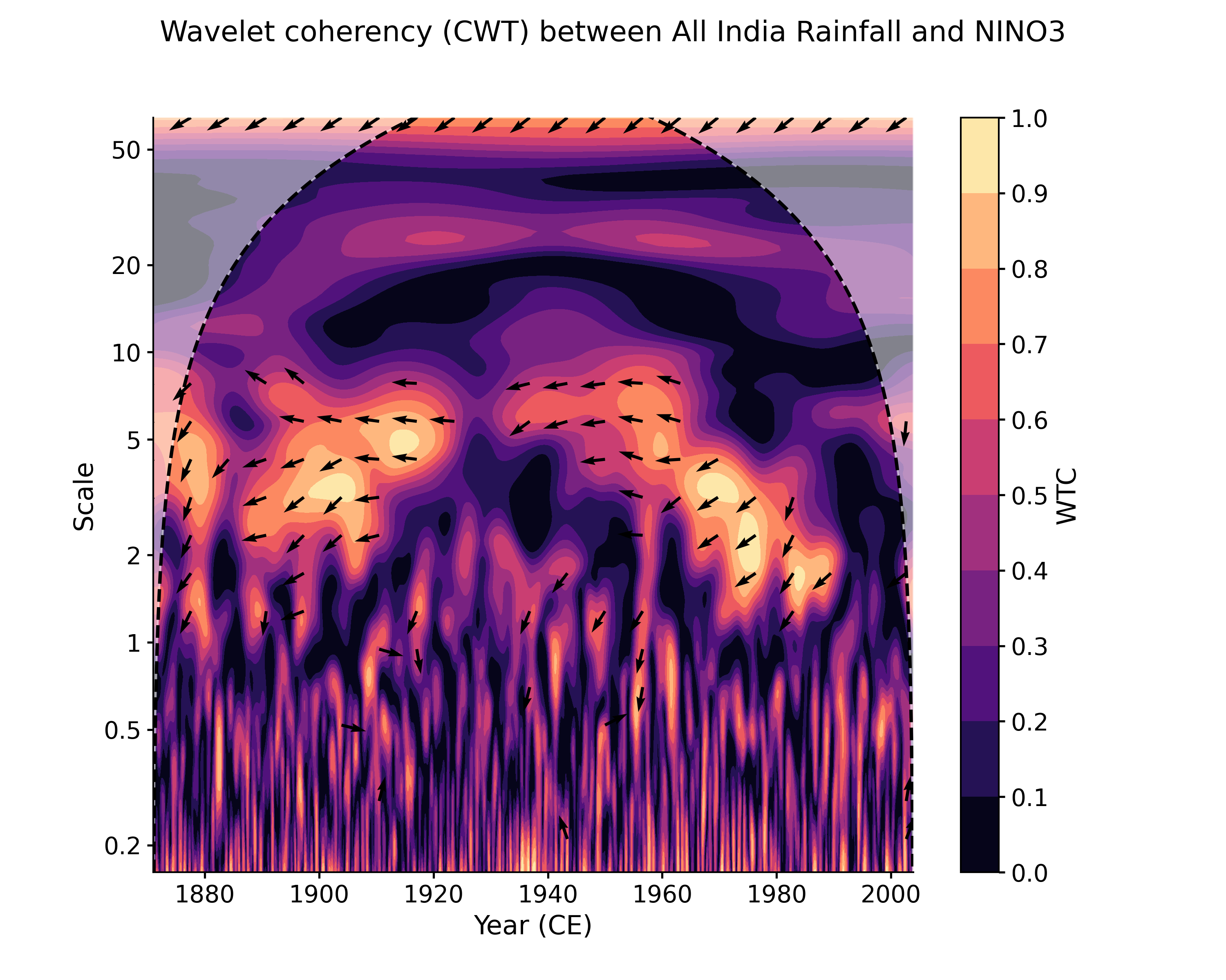
Establish significance against an AR(1) benchmark:

In [13]: coh_sig = coh.signif_test(number=20, qs=[.9,.95,.99])

In [14]: coh_sig.plot()
Out[14]: 
(<Figure size 1000x800 with 2 Axes>,
 <AxesSubplot: title={'center': 'Lines:95% threshold'}, xlabel='Year (CE)', ylabel='Scale'>)

In [15]: pyleo.closefig(fig)

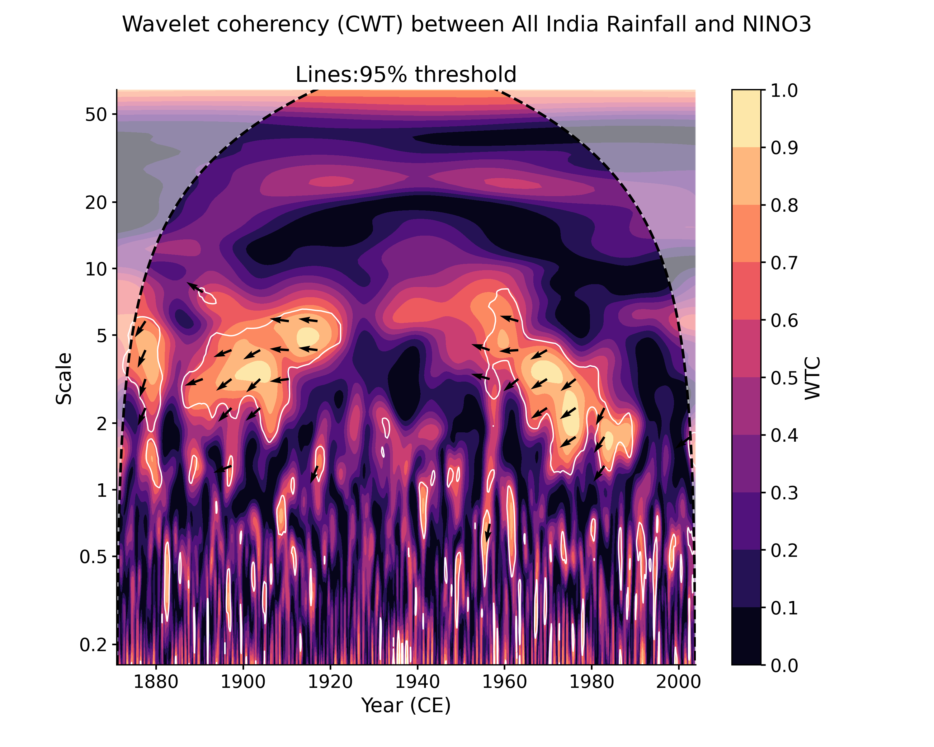
Note that specifiying 3 significance thresholds does not take any more time as the quantiles are simply estimated from the same ensemble. By default, the plot function looks for the closest quantile to 0.95, but this is easy to adjust, e.g. for the 99th percentile:

In [16]: coh_sig.plot(signif_thresh = 0.99)
Out[16]: 
(<Figure size 1000x800 with 2 Axes>,
 <AxesSubplot: title={'center': 'Lines:99% threshold'}, xlabel='Year (CE)', ylabel='Scale'>)

In [17]: pyleo.closefig(fig)

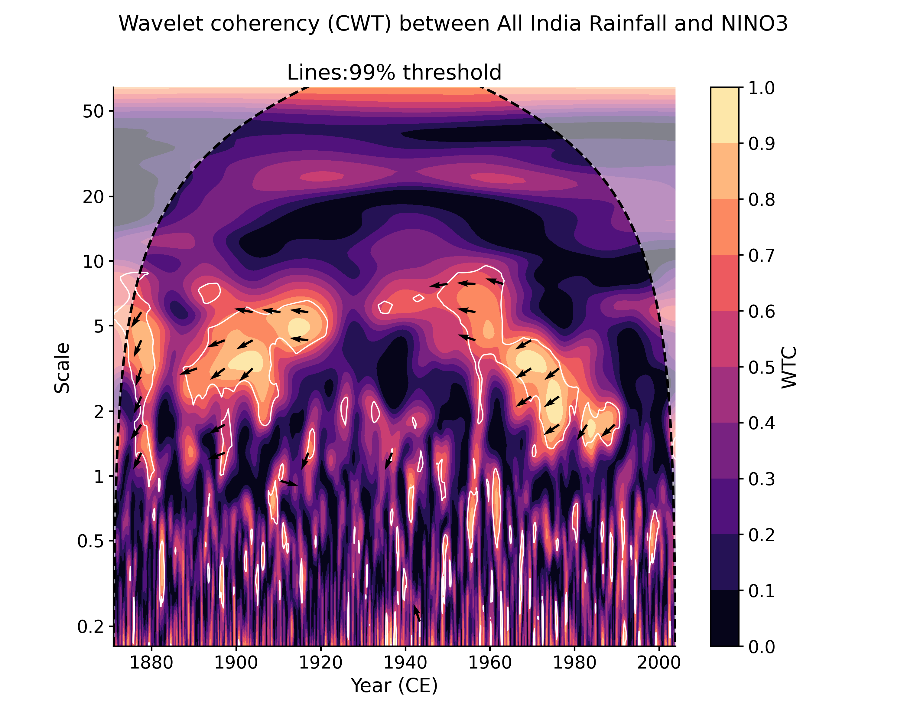
By default, the function plots the wavelet transform coherency (WTC), which quantifies where two timeseries exhibit similar behavior in time-frequency space, regardless of whether this corresponds to regions of high common power. To visualize the latter, you want to plot the cross-wavelet transform (XWT) instead, like so:

In [18]: coh_sig.plot(var='xwt')
Out[18]: 
(<Figure size 1000x800 with 2 Axes>,
 <AxesSubplot: title={'center': 'Lines:95% threshold'}, xlabel='Year (CE)', ylabel='Scale'>)

In [19]: pyleo.closefig(fig)

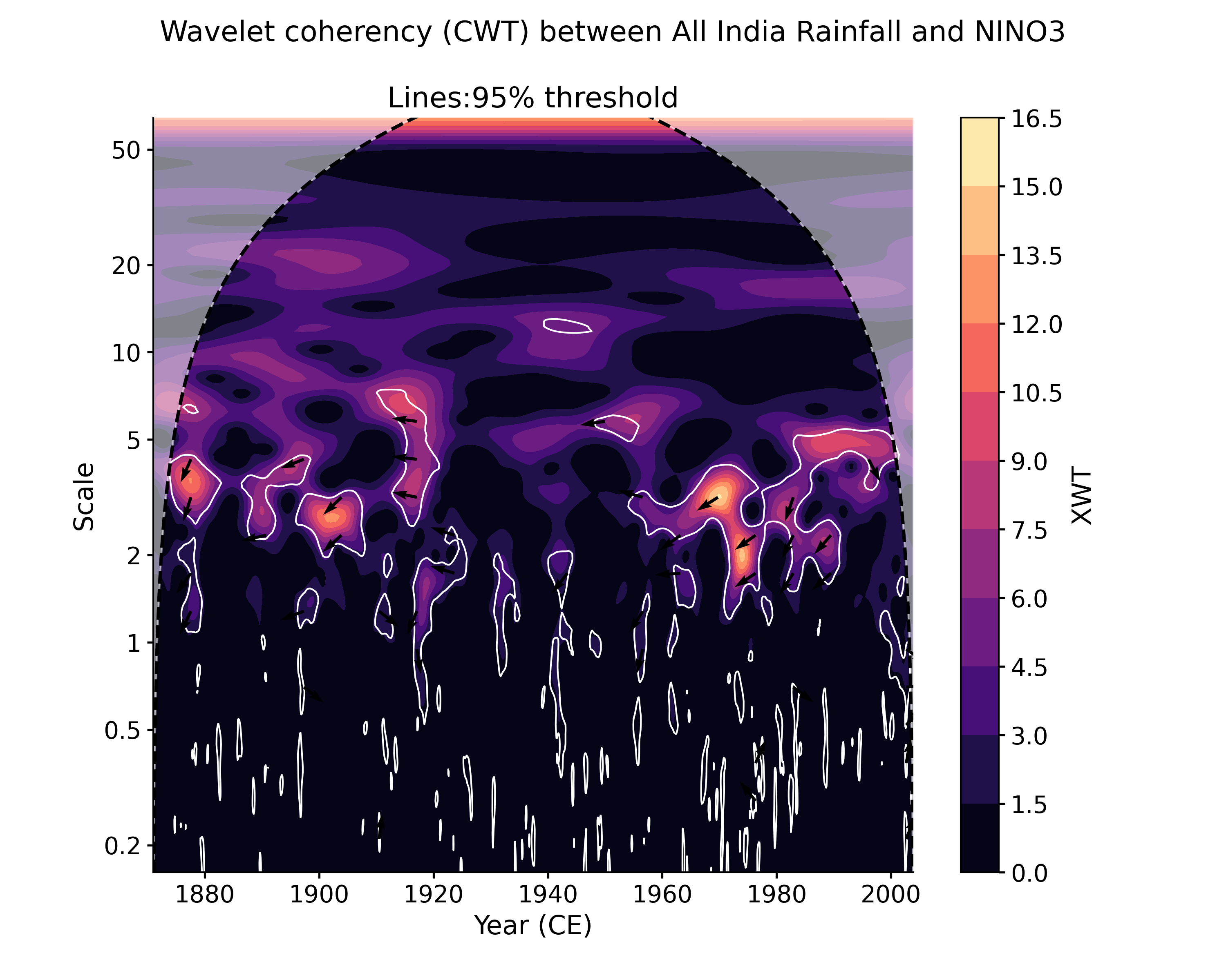
signif_test(number=200, method='ar1sim', seed=None, qs=[0.95], settings=None, mute_pbar=False)[source]

Significance testing for Coherence objects

The method obtains quantiles qs of the distribution of coherence between number pairs of Monte Carlo simulations of a process that resembles the original series. Currently, only AR(1) surrogates are supported.

Parameters:

number (int, optional) – Number of surrogate series to create for significance testing. The default is 200.
method ({'ar1sim'}, optional) – Method through which to generate the surrogate series. The default is ‘ar1sim’.
seed (int, optional) – Fixes the seed for NumPy’s random number generator. Useful for reproducibility. The default is None, so fresh, unpredictable entropy will be pulled from the operating system.
qs (list, optional) – Significance levels to return. The default is [0.95].
settings (dict, optional) – Parameters for surrogate model. The default is None.
mute_pbar (bool, optional) – Mute the progress bar. The default is False.

Returns:

new – original Coherence object augmented with significance levels signif_qs, a list with the following MultipleScalogram objects: * 0: MultipleScalogram for the wavelet transform coherency (WTC) * 1: MultipleScalogram for the cross-wavelet transform (XWT)

Each object contains as many Scalogram objects as qs contains values

Return type:

pyleoclim.core.coherence.Coherence

See also

pyleoclim.core.series.Series.wavelet_coherence: Wavelet coherence
pyleoclim.core.scalograms.Scalogram: Scalogram object
pyleoclim.core.scalograms.MultipleScalogram: Multiple Scalogram object
pyleoclim.core.coherence.Coherence.plot: plotting method for Coherence objects

Examples

Calculate the coherence of NINO3 and All India Rainfall and assess significance:

In [1]: import pyleoclim as pyleo

In [2]: import pandas as pd

In [3]: import numpy as np

In [4]: data = pd.read_csv('https://raw.githubusercontent.com/LinkedEarth/Pyleoclim_util/Development/example_data/wtc_test_data_nino_even.csv')

In [5]: time = data['t'].values

In [6]: air = data['air'].values

In [7]: nino = data['nino'].values

In [8]: ts_air = pyleo.Series(time=time, value=air, time_name='Year (CE)',
   ...:                       label='All India Rainfall', value_name='AIR (mm/month)')
   ...: 

In [9]: ts_nino = pyleo.Series(time=time, value=nino, time_name='Year (CE)',
   ...:                        label='NINO3', value_name='NINO3 (K)')
   ...: 

In [10]: coh = ts_air.wavelet_coherence(ts_nino)

In [11]: coh_sig = coh.signif_test(number=20)

In [12]: coh_sig.plot()
Out[12]: 
(<Figure size 1000x800 with 2 Axes>,
 <AxesSubplot: title={'center': 'Lines:95% threshold'}, xlabel='Year (CE)', ylabel='Scale'>)

In [13]: pyleo.closefig(fig)

By default, significance is assessed against a 95% benchmark derived from an AR(1) process fit to the data, using 200 Monte Carlo simulations. To customize, one can increase the number of simulations (more reliable, but slower), and the quantile levels.

In [14]: coh_sig2 = coh.signif_test(number=100, qs=[.9,.95,.99])

In [15]: coh_sig2.plot()
Out[15]: 
(<Figure size 1000x800 with 2 Axes>,
 <AxesSubplot: title={'center': 'Lines:95% threshold'}, xlabel='Year (CE)', ylabel='Scale'>)

In [16]: pyleo.closefig(fig)

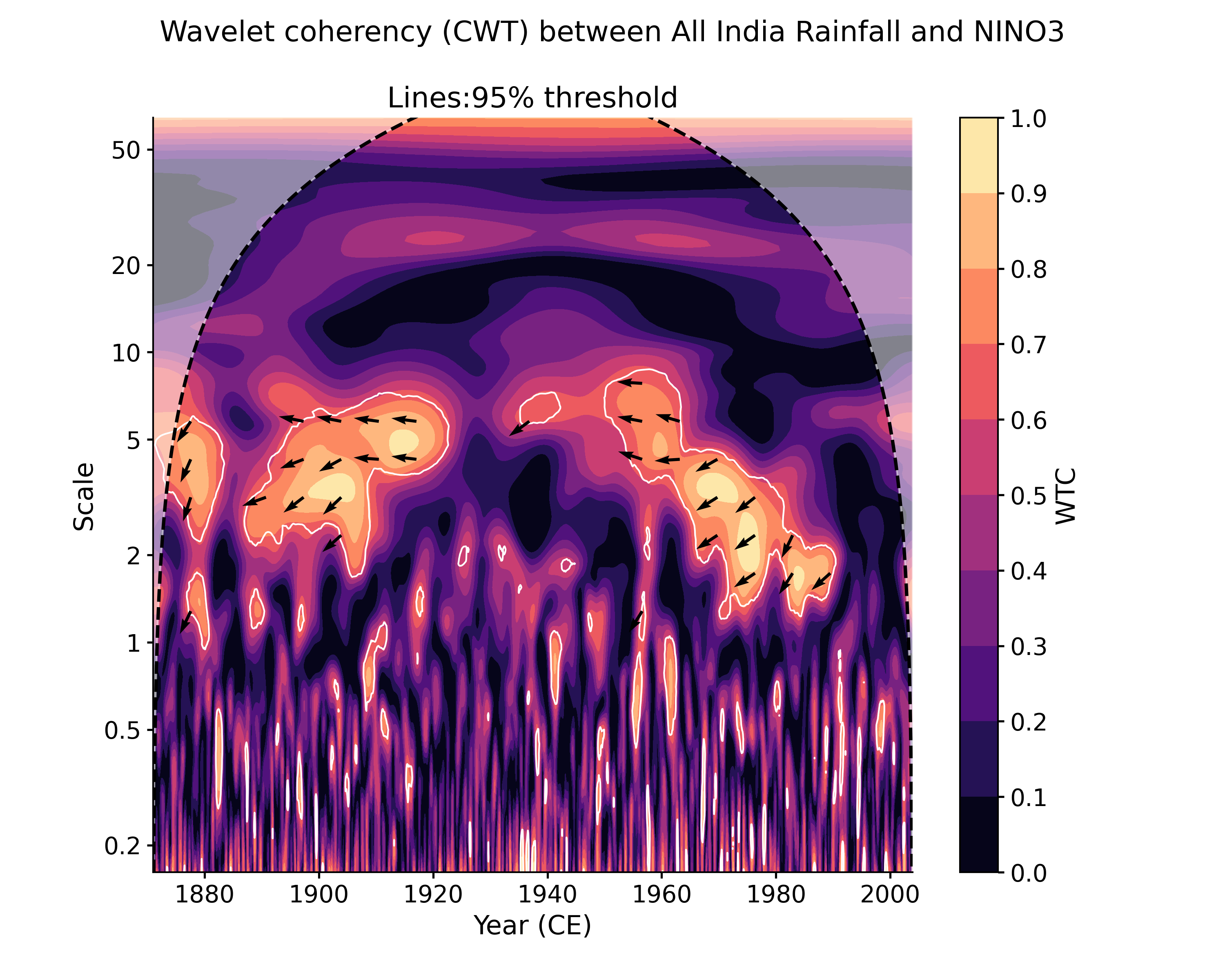
The plot() function will represent the 95% level as contours by default. If you need to show 99%, say, use the signif_thresh argument:

In [17]: coh_sig2.plot(signif_thresh=0.99)
Out[17]: 
(<Figure size 1000x800 with 2 Axes>,
 <AxesSubplot: title={'center': 'Lines:99% threshold'}, xlabel='Year (CE)', ylabel='Scale'>)

In [18]: pyleo.closefig(fig)

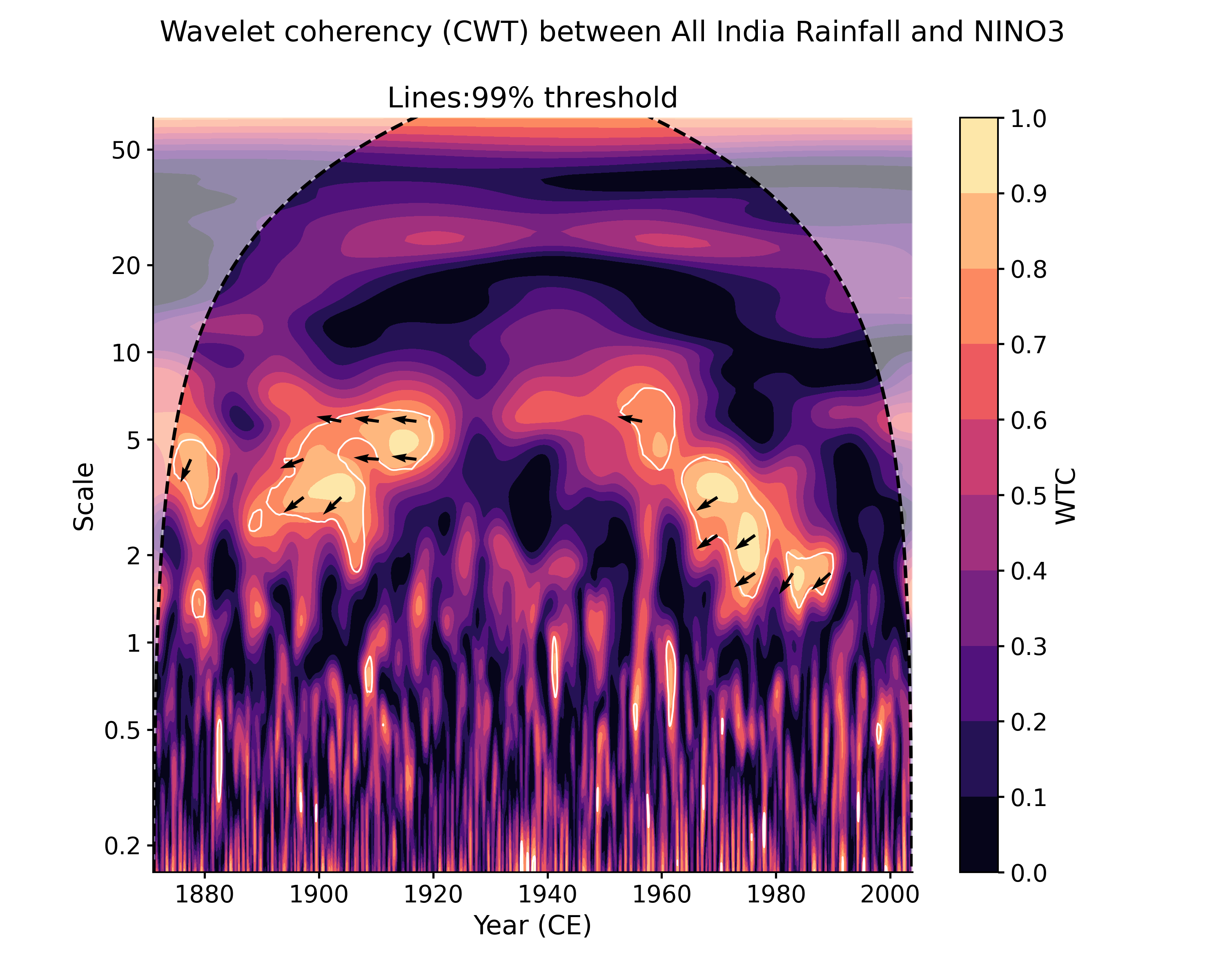
Note that if the 99% quantile is not present, the plot method will look for the closest match, but lines are always labeled appropriately. For reproducibility purposes, it may be good to specify the (pseudo)random number generator’s seed, like so:

In [19]: coh_sig27 = coh.signif_test(number=20, seed=27)

This will generate exactly the same set of draws from the (pseudo)random number at every execution, which may be important for marginal features in small ensembles. In general, however, we recommend increasing the number of draws to check that features are robust.

Corr (pyleoclim.Corr)

class pyleoclim.core.corr.Corr(r, p, signif, alpha, p_fmt_td=0.01, p_fmt_style='exp')[source]

The object for correlation results in order to format the print message

Parameters:

r (float) – the correlation coefficient
p (float) – the p-value
p_fmt_td (float) – the threshold for p-value formatting (0.01 by default, i.e., if p<0.01, will print “< 0.01” instead of “0”)
p_fmt_style (str) – the style for p-value formatting (exponential notation by default)
signif (bool) – the significance
alpha (float) – The significance level (0.05 by default)

See also

pyleoclim.utils.correlation.corr_sig: Correlation function
pyleoclim.utils.correlation.fdr: FDR function

Methods

copy()

Copy object

copy()[source]: Copy object

CorrEns (pyleoclim.CorrEns)

class pyleoclim.core.correns.CorrEns(r, p, signif, signif_fdr, alpha, p_fmt_td=0.01, p_fmt_style='exp')[source]

CorrEns objects store the result of an ensemble correlation calculation between timeseries and/or ensemble of timeseries. The class enables a print and plot function to easily visualize the result.

Parameters:

r (list) – the list of correlation coefficients
p (list) – the list of p-values
p_fmt_td (float) – the threshold for p-value formating (0.01 by default, i.e., if p<0.01, will print “< 0.01” instead of “0”)
p_fmt_style (str) – the style for p-value formating (exponential notation by default)
signif (list) – the list of significance without FDR
signif_fdr (list) – the list of significance with FDR
signif_fdr – the list of significance with FDR
alpha (float) – The significance level

See also

pyleoclim.utils.correlation.corr_sig: Correlation function
pyleoclim.utils.correlation.fdr: FDR (False Discovery Rate) function

Methods

`copy`()	Copy object
`plot`([figsize, title, ax, savefig_settings, ...])	Plot the distribution of correlation values as a histogram

copy()[source]: Copy object

plot(figsize=[4, 4], title=None, ax=None, savefig_settings=None, hist_kwargs=None, title_kwargs=None, xlim=None, alpha=0.8, multiple='layer', clr_insignif='silver', clr_signif='#029386', clr_signif_fdr='darkorange', clr_percentile='#ff796c')[source]

Plot the distribution of correlation values as a histogram

Uses seaborn’s histplot

Color-coding is used to indicate significance, with or without applying the False Discovery Rate (FDR) method.

Parameters:

figsize (list, optional) – The figure size. The default is [4, 4].
title (str, optional) – Plot title. The default is None.
multiple (str, optional) – Approach to organizing the 3 different histrograms on the plot. possible values: “layer”[default], “dodge”, “stack”, “fill”
alpha (float in [0, 1]) – transparency parameter for histrogram bars. Default: 0.8
savefig_settings (dict) –
the dictionary of arguments for plt.savefig(); some notes below: - “path” must be specified; it can be any existing or new path,

with or without a suffix; if the suffix is not given in “path”, it will follow “format”
- ”format” can be one of {“pdf”, “eps”, “png”, “ps”}
hist_kwargs (dict) – additional keyword arguments for sns.histplot() [experimental]
title_kwargs (dict) – the keyword arguments for ax.set_title()
ax (matplotlib.axis, optional) – the axis object from matplotlib See [matplotlib.axes](https://matplotlib.org/api/axes_api.html) for details.
xlim (list, optional) – x-axis limits. The default is None.

See also

pyleoclim.core.series.Series.correlation: correlation with significance
pyleoclim.utils.correlation.fdr: False Discovery Rate
seaborn.histplot: https://seaborn.pydata.org/generated/seaborn.histplot.html
pyleoclim.utils.plotting.savefig: save figures in Pyleoclim

SpatialDecomp (pyleoclim.SpatialDecomp)

class pyleoclim.core.spatialdecomp.SpatialDecomp(time, locs, name, eigvals, eigvecs, pctvar, pcs, neff)[source]

Class to hold the results of spatial decompositions applies to : pca(), mcpca(), mssa()

Parameters:

time (float) – the common time axis
locs (float (p, 2)) – a p x 2 array of coordinates (latitude, longitude) for mapping the spatial patterns (“EOFs”)
name (str) – name of the dataset/analysis to use in plots
eigvals (float) – vector of eigenvalues from the decomposition
eigvecs (float) – array of eigenvectors from the decomposition
pctvar (float) – array of pct variance accounted for by each mode
neff (float) – scalar representing the effective sample size of the leading mode

Methods

`modeplot`([index, figsize, ax, ...])	Dashboard visualizing the properties of a given mode, including:
`screeplot`([figsize, uq, title, ax, ...])	Plot the eigenvalue spectrum with uncertainties

modeplot(index=0, figsize=[10, 5], ax=None, savefig_settings=None, title_kwargs=None, spec_method='mtm')[source]

Dashboard visualizing the properties of a given mode, including:

The temporal coefficient (PC or similar)
its spectrum
The spatial loadings (EOF or similar)

Parameters:

index (int) – the (0-based) index of the mode to visualize. Default is 0, corresponding to the first mode.
figsize (list, optional) – The figure size. The default is [10, 5].
savefig_settings (dict) –
the dictionary of arguments for plt.savefig(); some notes below: - “path” must be specified; it can be any existed or non-existed path,

with or without a suffix; if the suffix is not given in “path”, it will follow “format”
- ”format” can be one of {“pdf”, “eps”, “png”, “ps”}
title_kwargs (dict) – the keyword arguments for ax.set_title()
gs (matplotlib.gridspec object, optional) – the axis object from matplotlib See [matplotlib.gridspec.GridSpec](https://matplotlib.org/stable/tutorials/intermediate/gridspec.html) for details.
spec_method (str, optional) – The name of the spectral method to be applied on the PC. Default: MTM Note that the data are evenly-spaced, so any spectral method that assumes even spacing is applicable here: ‘mtm’, ‘welch’, ‘periodogram’ ‘wwz’ is relevant if scaling exponents need to be estimated, but ill-advised otherwise, as it is very slow.

screeplot(figsize=[6, 4], uq='N82', title='scree plot', ax=None, savefig_settings=None, title_kwargs=None, xlim=[0, 10], clr_eig='C0')[source]

Plot the eigenvalue spectrum with uncertainties

Parameters:

figsize (list, optional) – The figure size. The default is [6, 4].
title (str, optional) – Plot title. The default is ‘scree plot’.
savefig_settings (dict) –
the dictionary of arguments for plt.savefig(); some notes below: - “path” must be specified; it can be any existed or non-existed path,

with or without a suffix; if the suffix is not given in “path”, it will follow “format”
- ”format” can be one of {“pdf”, “eps”, “png”, “ps”}
title_kwargs (dict, optional) – the keyword arguments for ax.set_title()
ax (matplotlib.axis, optional) – the axis object from matplotlib See [matplotlib.axes](https://matplotlib.org/api/axes_api.html) for details.
xlim (list, optional) – x-axis limits. The default is [0, 10] (first 10 eigenvalues)
uq (str, optional) – Method used for uncertainty quantification of the eigenvalues. ‘N82’ uses the North et al “rule of thumb” [1] with effective sample size computed as in [2]. ‘MC’ uses Monte-Carlo simulations (e.g. MC-EOF). Returns an error if no ensemble is found.
clr_eig (str, optional) – color to be used for plotting eigenvalues

References

[1]_ North, G. R., T. L. Bell, R. F. Cahalan, and F. J. Moeng (1982), Sampling errors in the estimation of empirical orthogonal functions, Mon. Weather Rev., 110, 699–706.

[2]_ Hannachi, A., I. T. Jolliffe, and D. B. Stephenson (2007), Empirical orthogonal functions and related techniques in atmospheric science: A review, International Journal of Climatology, 27(9), 1119–1152, doi:10.1002/joc.1499.

SsaRes (pyleoclim.SsaRes)

class pyleoclim.core.ssares.SsaRes(time, original, name, eigvals, eigvecs, pctvar, PC, RCmat, RCseries, mode_idx, eigvals_q=None)[source]

This class is meant to hold the output of the Singular Spectrum Analysis (SSA) method, which applies to Series objets. Two functions are enabled by this class:

screeplot, which plots the eigenvalue spectrum to help determine what modes to keep
modeplot, which plots the individual mode temporal EOF and temporal PC

Parameters:

eigvals (float (M, 1)) – a vector of real eigenvalues derived from the signal
pctvar (float (M, 1)) – same vector, expressed in % variance accounted for by each mode.
eigvals_q (float (M, 2)) – array containing the 5% and 95% quantiles of the Monte-Carlo eigenvalue spectrum [ assigned NaNs if unused ]
eigvecs (float (M, M)) – a matrix of the temporal eigenvectors (T-EOFs), i.e. the temporal patterns that explain most of the variations in the original series.
PC (float (N - M + 1, M)) – array of principal components, i.e. the loadings that, convolved with the T-EOFs, produce the reconstructed components, or RCs
RCmat (float (N, M)) – array of reconstructed components, One can think of each RC as the contribution of each mode to the timeseries, weighted by their eigenvalue (loosely speaking, their “amplitude”). Summing over all columns of RC recovers the original series. (synthesis, the reciprocal operation of analysis).
mode_idx (list) – index of retained modes
RCseries (float (N, 1)) – reconstructed series based on the RCs of mode_idx (scaled to original series; mean must be added after the fact)

See also

pyleoclim.utils.decomposition.ssa: Singular Spectrum Analysis

Methods

`copy`()	Make a copy of the SsaRes object
`modeplot`([index, figsize, savefig_settings, ...])	Dashboard visualizing the properties of a given SSA mode, including:
`screeplot`([figsize, title, ax, ...])	Scree plot for SSA, visualizing the eigenvalue spectrum and indicating which modes were retained.

copy()[source]

Make a copy of the SsaRes object

Returns:: SsaRes – A copy of the SsaRes object
Return type:: pyleoclim.SsaRes

modeplot(index=0, figsize=[10, 5], savefig_settings=None, title_kwargs=None, spec_method='mtm', plot_original=True)[source]

Dashboard visualizing the properties of a given SSA mode, including:

the analyzing function (T-EOF)
the reconstructed component (RC)
its spectrum

Parameters:

index (int) – the (0-based) index of the mode to visualize. Default is 0, corresponding to the first mode.
figsize (list, optional) – The figure size. The default is [10, 5].
savefig_settings (dict) –
the dictionary of arguments for plt.savefig(); some notes below: - “path” must be specified; it can be any existed or non-existed path,

with or without a suffix; if the suffix is not given in “path”, it will follow “format”
- ”format” can be one of {“pdf”, “eps”, “png”, “ps”}
title_kwargs (dict) – the keyword arguments for ax.set_title()
spec_method (str, optional) – The name of the spectral method to be applied on the PC. Default: MTM Note that the data are evenly-spaced, so any spectral method that assumes even spacing is applicable here: ‘mtm’, ‘welch’, ‘periodogram’. ‘wwz’ is relevant too if scaling exponents need to be estimated.

See also

pyleoclim.core.series.Series.ssa: Singular Spectrum Analysis for timeseries objects
pyleoclim.utils.decomposition.ssa: Singular Spectrum Analysis utility
pyleoclim.core.ssares.SsaRes.screeplot: plot SSA eigenvalue spectrum

Examples

Plot the first SSA mode of the Southern Oscillation Index:

In [1]: data = pd.read_csv('https://raw.githubusercontent.com/LinkedEarth/Pyleoclim_util/Development/example_data/soi_data.csv',skiprows=0,header=1)

In [2]: ts = pyleo.Series(time=data.iloc[:,1], value=data.iloc[:,2], time_name='Year C.E', value_name='SOI', label='SOI')

In [3]: ssa = ts.ssa()

In [4]: fig, ax = ssa.modeplot()

In [5]: pyleo.closefig(fig)

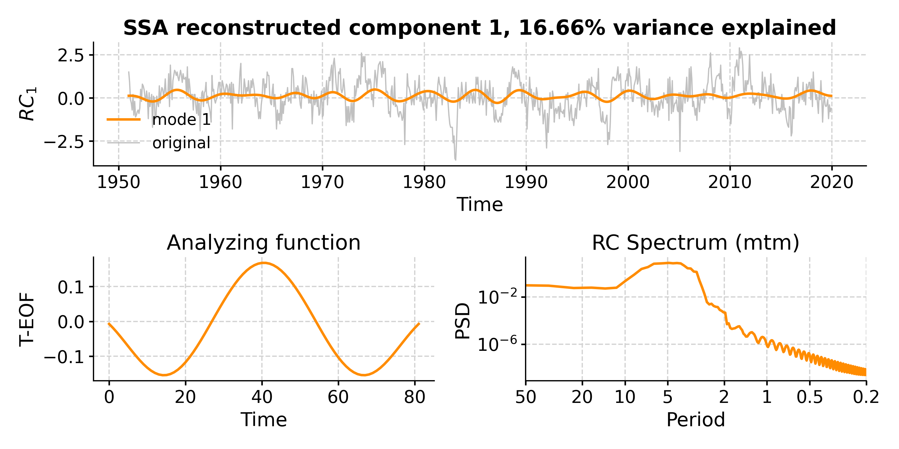
Plot the second mode (note 0-based indexing):

In [6]: fig, ax = ssa.modeplot(index=1)

In [7]: pyleo.closefig(fig)

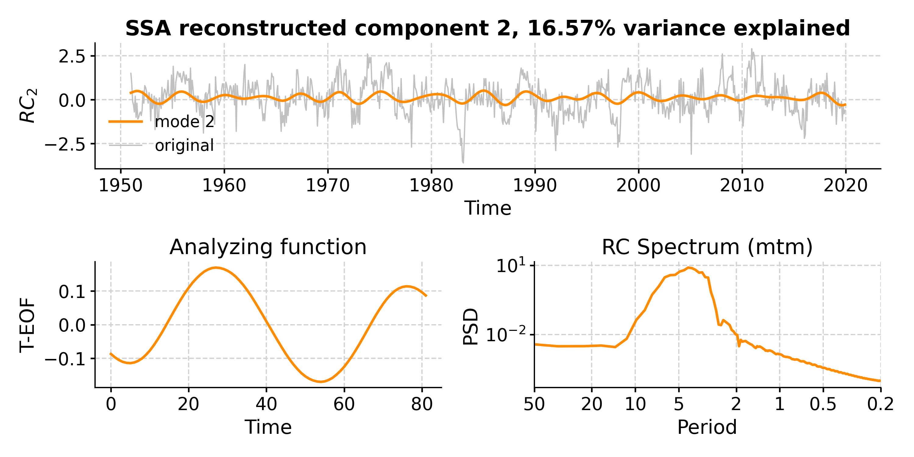
screeplot(figsize=[6, 4], title='SSA scree plot', ax=None, savefig_settings=None, title_kwargs=None, xlim=None, clr_mcssa='#e50000', clr_signif='#029386', clr_eig='black')[source]

Scree plot for SSA, visualizing the eigenvalue spectrum and indicating which modes were retained.

Parameters:

figsize (list, optional) – The figure size. The default is [6, 4].
title (str, optional) – Plot title. The default is ‘SSA scree plot’.
savefig_settings (dict) –
the dictionary of arguments for plt.savefig(); some notes below:
- ”path” must be specified; it can be any existed or non-existed path, with or without a suffix; if the suffix is not given in “path”, it will follow “format”
- ”format” can be one of {“pdf”, “eps”, “png”, “ps”}
title_kwargs (dict) – the keyword arguments for ax.set_title()
ax (matplotlib.axis, optional) – the axis object from matplotlib See [matplotlib.axes](https://matplotlib.org/api/axes_api.html) for details.
xlim (list, optional) – x-axis limits. The default is None.
clr_mcssa (str, optional) – color of the Monte Carlo SSA AR(1) shading (if data are provided) default: red
clr_eig (str, optional) – color of the eigenvalues, default: black
clr_signif (str, optional) – color of the highlights for significant eigenvalue. (default: teal)

See also

pyleoclim.core.series.Series.ssa: Singular Spectrum Analysis for timeseries objects
pyleoclim.core.utils.decomposition.ssa: Singular Spectrum Analysis utility
pyleoclim.core.ssares.SsaRes.modeplot: plot SSA modes

Examples

Plot the SSA eigenvalue spectrum of the Southern Oscillation Index:

In [1]: data = pd.read_csv('https://raw.githubusercontent.com/LinkedEarth/Pyleoclim_util/Development/example_data/soi_data.csv',skiprows=0,header=1)

In [2]: ts = pyleo.Series(time=data.iloc[:,1], value=data.iloc[:,2], time_name='Year C.E', value_name='SOI', label='SOI')

In [3]: ssa = ts.ssa()

In [4]: fig, ax = ssa.screeplot()

In [5]: pyleo.closefig(fig)