Pyleoclim Utilities API (pyleoclim.utils)

Utilities upon which Pyleoclim depends for higher-level functionalities accessible to users.

Pyleoclim makes extensive use of functions from numpy, Pandas, Scipy, Matplotlib, Statsmodels, and scikit-learn. Please note that some default parameter values for these functions have been changed to values more appropriate for paleoclimate datasets.

Causality

Utilities for Liang and Granger causality analysis

pyleoclim.utils.causality.granger_causality(y1, y2, maxlag=1, addconst=True, verbose=True)[source]

Granger causality tests

Four tests for the Granger non-causality of 2 time series.

All four tests give similar results. params_ftest and ssr_ftest are equivalent based on F test which is identical to lmtest:grangertest in R.

Wrapper for the functions described in statsmodel (https://www.statsmodels.org/stable/generated/statsmodels.tsa.stattools.grangercausalitytests.html)

Parameters

y1 (array) – vectors of (real) numbers with identical length, no NaNs allowed
y2 (array) – vectors of (real) numbers with identical length, no NaNs allowed
maxlag (int or int iterable, optional) – If an integer, computes the test for all lags up to maxlag. If an iterable, computes the tests only for the lags in maxlag.
addconst (bool, optional) – Include a constant in the model.
verbose (bool, optional) – Print results

Returns

All test results, dictionary keys are the number of lags. For each lag the values are a tuple, with the first element a dictionary with test statistic, pvalues, degrees of freedom, the second element are the OLS estimation results for the restricted model, the unrestricted model and the restriction (contrast) matrix for the parameter f_test.

Return type

dict

Notes

The null hypothesis for Granger causality tests is that the time series in the second column, x2, does NOT Granger cause the time series in the first column, x1. Grange causality means that past values of x2 have a statistically significant effect on the current value of x1, taking past values of x1 into account as regressors. We reject the null hypothesis that x2 does not Granger cause x1 if the pvalues are below a desired size of the test.

The null hypothesis for all four test is that the coefficients corresponding to past values of the second time series are zero.

‘params_ftest’, ‘ssr_ftest’ are based on F distribution

‘ssr_chi2test’, ‘lrtest’ are based on chi-square distribution

See also

pyleoclim.utils.causality.liang_causality: information flow estimated using the Liang algorithm
pyleoclim.utils.causality.signif_isopersist: significance test with AR(1) with same persistence
pyleoclim.utils.causality.signif_isospec: significance test with surrogates with randomized phases

References

Granger, C. W. J. (1969). Investigating causal relations by econometric models and cross-spectral methods. Econometrica, 37(3), 424-438.

Granger, C. W. J. (1980). Testing for causality: A personal viewpoont. Journal of Economic Dynamics and Control, 2, 329-352.

Granger, C. W. J. (1988). Some recent development in a concept of causality. Journal of Econometrics, 39(1-2), 199-211.

pyleoclim.utils.causality.liang_causality(y1, y2, npt=1, signif_test='isospec', nsim=1000, qs=[0.005, 0.025, 0.05, 0.95, 0.975, 0.995])[source]

Liang-Kleeman information flow

Estimate the Liang information transfer from series y2 to series y1 with significance estimates using either an AR(1) tests with series with the same persistence or surrogates with randomized phases.

Parameters

y1 (array) – vectors of (real) numbers with identical length, no NaNs allowed
y2 (array) – vectors of (real) numbers with identical length, no NaNs allowed
npt (int >=1) – time advance in performing Euler forward differencing, e.g., 1, 2. Unless the series are generated with a highly chaotic deterministic system, npt=1 should be used
signif_test (str; {'isopersist', 'isospec'}) – the method for significance test see signif_isospec and signif_isopersist for details.
nsim (int) – the number of AR(1) surrogates for significance test
qs (list) – the quantiles for significance test

Returns

res –

A dictionary of results including:

T21float: information flow from y2 to y1 (Note: not y1 -> y2!)
tau21float: the standardized information flow from y2 to y1
Zfloat: the total information flow from y2 to y1
dH1_starfloat: dH*/dt (Liang, 2016)

dH1_noise : float signif_qs :

the quantiles for significance test

T21_noiselist: the quantiles of the information flow from noise2 to noise1 for significance testing
tau21_noiselist: the quantiles of the standardized information flow from noise2 to noise1 for significance testing

Return type

dict

See also

pyleoclim.utils.causality.liang: information flow estimated using the Liang algorithm
pyleoclim.utils.causality.granger_causality: information flow estimated using the Granger algorithm
pyleoclim.utils.causality.signif_isopersist: significance test with AR(1) with same persistence
pyleoclim.utils.causality.causality.signif_isospec: significance test with surrogates with randomized phases

References

Liang, X.S. (2013) The Liang-Kleeman Information Flow: Theory and Applications. Entropy, 15, 327-360, doi:10.3390/e15010327

Liang, X.S. (2014) Unraveling the cause-effect relation between timeseries. Physical review, E 90, 052150

Liang, X.S. (2015) Normalizing the causality between time series. Physical review, E 92, 022126

Liang, X.S. (2016) Information flow and causality as rigorous notions ab initio. Physical review, E 94, 052201

Correlation

Relevant functions for correlation analysis

pyleoclim.utils.correlation.corr_sig(y1, y2, nsim=1000, method='isospectral', alpha=0.05)[source]

Estimates the Pearson’s correlation and associated significance between two non IID time series

The significance of the correlation is assessed using one of the following methods:

‘ttest’: T-test adjusted for effective sample size.
This is a parametric test (data are Gaussian and identically distributed) with a rather ad-hoc adjustment. It is instantaneous but makes a lot of assumptions about the data, many of which may not be met.
‘isopersistent’: AR(1) modeling of x and y.
This is a parametric test as well (series follow an AR(1) model) but solves the issue by direct simulation.
‘isospectral’: phase randomization of original inputs. (default)
This is a non-parametric method, assuming only wide-sense stationarity

For 2 and 3, computational requirements scale with nsim. When possible, nsim should be at least 1000.

Parameters

y1 (array) – vector of (real) numbers of same length as y2, no NaNs allowed
y2 (array) – vector of (real) numbers of same length as y1, no NaNs allowed
nsim (int) – the number of simulations [default: 1000]
method (str; {'ttest','isopersistent','isospectral' (default)}) – method for significance testing
alpha (float) – significance level for critical value estimation [default: 0.05]

Returns

res – the result dictionary, containing

rfloat
correlation coefficient
pfloat
the p-value
signifbool
true if significant; false otherwise Note that signif = True if and only if p <= alpha.

Return type

dict

See also

pyleoclim.utils.correlation.corr_ttest: Estimates the significance of correlations between 2 time series using the classical T-test adjusted for effective sample size
pyleoclim.utils.correlation.corr_isopersist: Computes correlation between two timeseries, and their significance using Ar(1) modeling
pyleoclim.utils.correlation.corr_isospec: Estimates the significance of the correlation using phase randomization
pyleoclim.utils.correlation.fdr: Determine significance based on the false discovery rate

pyleoclim.utils.correlation.fdr(pvals, qlevel=0.05, method='original', adj_method=None, adj_args={})[source]

Determine significance based on the false discovery rate

The false discovery rate is a method of conceptualizing the rate of type I errors in null hypothesis testing when conducting multiple comparisons. Translated from fdr.R by Dr. Chris Paciorek

Parameters

pvals (list or array) – A vector of p-values on which to conduct the multiple testing.
qlevel (float) – The proportion of false positives desired.
method ({'original', 'general'}) –
Method for performing the testing.
- ’original’ follows Benjamini & Hochberg (1995);
- ’general’ is much more conservative, requiring no assumptions on the p-values (see Benjamini & Yekutieli (2001)).
’original’ is recommended, and if desired, using ‘adj_method=”mean”’ to increase power.
adj_method ({'mean', 'storey', 'two-stage'}) –
Method for increasing the power of the procedure by estimating the proportion of alternative p-values.
- ’mean’, the modified Storey estimator in Ventura et al. (2004)
- ’storey’, the method of Storey (2002)
- ’two-stage’, the iterative approach of Benjamini et al. (2001)
adj_args (dict) – Arguments for adj_method; see prop_alt() for description, but note that for “two-stage”, qlevel and fdr_method are taken from the qlevel and method arguments for fdr()

Returns

fdr_res – A vector of the indices of the significant tests; None if no significant tests

Return type

array or None

See also

pyleoclim.utils.correlation.corr_sig: Estimates the Pearson’s correlation and associated significance between two non IID time series

References

fdr.R by Dr. Chris Paciorek: https://www.stat.berkeley.edu/~paciorek/research/code/code.html

Decomposition

Eigendecomposition methods: Singular Spectrum Analysis (SSA). soon: Monte-Carlo Principal Component Analysis, Multi-Channel SSA

pyleoclim.utils.decomposition.ssa(y, M=None, nMC=0, f=0.5, trunc=None, var_thresh=80)[source]

Singular spectrum analysis

Nonparametric eigendecomposition of timeseries into orthogonal oscillations. This implementation uses the method of [1], with applications presented in [2]. Optionally (nMC>0), the significance of eigenvalues is assessed by Monte-Carlo simulations of an AR(1) model fit to X, using [3]. The method expects regular spacing, but is tolerant to missing values, up to a fraction 0<f<1 (see [4]).

Parameters

y (array of length N) – time series (evenly-spaced, possibly with up to f*N NaNs)
M (int) – window size (default: 10% of N)
nMC (int) – Number of iterations in the Monte-Carlo simulation (default nMC=0, bypasses Monte Carlo SSA) Currently only supported for evenly-spaced, gap-free data.
f (float) – maximum allowable fraction of missing values. (Default is 0.5)
trunc (str) –
if present, truncates the expansion to a level K < M owing to one of 3 criteria:
1. ’kaiser’: variant of the Kaiser-Guttman rule, retaining eigenvalues larger than the median
2. ’mcssa’: Monte-Carlo SSA (use modes above the 95% quantile from an AR(1) process)
3. ’var’: first K modes that explain at least var_thresh % of the variance.
Default is None, which bypasses truncation (K = M)
var_thresh (float) – variance threshold for reconstruction (only impactful if trunc is set to ‘var’)

Returns

res –

eigvals : (M, ) array of eigenvalues
eigvecs : (M, M) Matrix of temporal eigenvectors (T-EOFs)
PC : (N - M + 1, M) array of principal components (T-PCs)
RCmat : (N, M) array of reconstructed components
RCseries : (N,) reconstructed series, with mean and variance restored
pctvar: (M, ) array of the fraction of variance (%) associated with each mode
eigvals_q : (M, 2) array containting the 5% and 95% quantiles of the Monte-Carlo eigenvalue spectrum [ if nMC >0 ]
mode_idx : array of indices of eigenvalues >=eigvals_q

Return type

dict containing:

References

[1]_ Vautard, R., and M. Ghil (1989), Singular spectrum analysis in nonlinear dynamics, with applications to paleoclimatic time series, Physica D, 35, 395–424.

[2]_ Ghil, M., R. M. Allen, M. D. Dettinger, K. Ide, D. Kondrashov, M. E. Mann, A. Robertson, A. Saunders, Y. Tian, F. Varadi, and P. Yiou (2002), Advanced spectral methods for climatic time series, Rev. Geophys., 40(1), 1003–1052, doi:10.1029/2000RG000092.

[3]_ Allen, M. R., and L. A. Smith (1996), Monte Carlo SSA: Detecting irregular oscillations in the presence of coloured noise, J. Clim., 9, 3373–3404.

[4]_ Schoellhamer, D. H. (2001), Singular spectrum analysis for time series with missing data, Geophysical Research Letters, 28(16), 3187–3190, doi:10.1029/2000GL012698.

See also

pyleoclim.core.series.Series.ssa: Singular Spectrum Analysis for timeseries objects
pyleoclim.core.ssares.SsaRes.modeplot: plot SSA modes
pyleoclim.core.ssares.SsaRes.screeplot: plot SSA eigenvalue spectrum

Filter

Utilities to filter arrayed timeseries data, leveraging SciPy

pyleoclim.utils.filter.butterworth(ys, fc, fs=1, filter_order=3, pad='reflect', reflect_type='odd', params=(1, 0, 0), padFrac=0.1)[source]

Applies a Butterworth filter with frequency fc, with padding: Supports both lowpass and band-pass filtering.

Parameters

ys (numpy array) – Timeseries
fc (float or list) – cutoff frequency. If scalar, it is interpreted as a low-frequency cutoff (lowpass) If fc is a list, it is interpreted as a frequency band (f1, f2), with f1 < f2 (bandpass)
fs (float) – sampling frequency
filter_order (int) – order n of Butterworth filter
pad (str) – Indicates if padding is needed. - ‘reflect’: Reflects the timeseries - ‘ARIMA’: Uses an ARIMA model for the padding - None: No padding.
params (tuple) – model parameters for ARIMA model (if pad = ‘ARIMA’)
padFrac (float) – fraction of the series to be padded

Returns

yf – filtered array

Return type

array

See also

pyleoclim.utils.filter.ts_pad: Pad a timeseries based on timeseries model predictions
pyleoclim.utils.filter.firwin: Applies a Finite Impulse Response filter with frequency fc, with padding
pyleoclim.utils.filter.savitzky_golay: Smooth (and optionally differentiate) data with a Savitzky-Golay filter
pyleoclim.utils.filter.lanczos: Applies a Lanczos filter with frequency fc, with padding

pyleoclim.utils.filter.firwin(ys, fc, numtaps=None, fs=1, pad='reflect', window='hamming', reflect_type='odd', params=(1, 0, 0), padFrac=0.1, **kwargs)[source]

Applies a Finite Impulse Response filter design with window method and frequency fc, with padding

Parameters

ys (numpy array) – Timeseries
fc (float or list) – cutoff frequency. If scalar, it is interpreted as a low-frequency cutoff (lowpass) If fc is a list, it is interpreted as a frequency band (f1, f2), with f1 < f2 (bandpass)
numptaps (int) – Length of the filter (number of coefficients, i.e. the filter order + 1). numtaps must be odd if a passband includes the Nyquist frequency. If None, will use the largest number that is smaller than 1/3 of the the data length.
fs (float) – sampling frequency
window (str or tuple of string and parameter values, optional) – Desired window to use. See scipy.signal.get_window for a list of windows and required parameters.
pad (str) – Indicates if padding is needed. - ‘reflect’: Reflects the timeseries - ‘ARIMA’: Uses an ARIMA model for the padding - None: No padding.
params (tuple) – model parameters for ARIMA model (if pad = True)
padFrac (float) – fraction of the series to be padded
kwargs (dict) – a dictionary of keyword arguments for scipy.signal.firwin

Returns

yf – filtered array

Return type

array

See also

scipy.signal.firwin: FIR filter design using the window method
pyleoclim.utils.filter.ts_pad: Pad a timeseries based on timeseries model predictions
pyleoclim.utils.filter.butterworth: Applies a Butterworth filter with frequency fc, with padding
pyleoclim.utils.filter.lanczos: Applies a Lanczos filter with frequency fc, with padding
pyleoclim.utils.filter.savitzky_golay: Smooth (and optionally differentiate) data with a Savitzky-Golay filter

pyleoclim.utils.filter.lanczos(ys, fc, fs=1, pad='reflect', reflect_type='odd', params=(1, 0, 0), padFrac=0.1)[source]

Applies a Lanczos (lowpass) filter with frequency fc, with optional padding

Parameters

ys (numpy array) – Timeseries
fc (float) – cutoff frequency
fs (float) – sampling frequency
pad (str) – Indicates if padding is needed - ‘reflect’: Reflects the timeseries - ‘ARIMA’: Uses an ARIMA model for the padding - None: No padding
params (tuple) – model parameters for ARIMA model (if pad = ‘ARIMA’). May require fiddling
padFrac (float) – fraction of the series to be padded

Returns

yf – filtered array

Return type

array

See also

pyleoclim.utils.filter.ts_pad: Pad a timeseries based on timeseries model predictions
pyleoclim.utils.filter.butterworth: Applies a Butterworth filter with frequency fc, with padding
pyleoclim.utils.filter.firwin: Applies a Finite Impulse Response filter with frequency fc, with padding
pyleoclim.utils.filter.savitzky_golay: Smooth (and optionally differentiate) data with a Savitzky-Golay filter

References

Filter design from http://scitools.org.uk/iris/docs/v1.2/examples/graphics/SOI_filtering.html

pyleoclim.utils.filter.savitzky_golay(ys, window_length=None, polyorder=2, deriv=0, delta=1, axis=-1, mode='mirror', cval=0)[source]

Smooth (and optionally differentiate) data with a Savitzky-Golay filter.

The Savitzky-Golay filter removes high frequency noise from data. It has the advantage of preserving the original shape and features of the signal better than other types of filtering approaches, such as moving averages techniques.

The Savitzky-Golay is a type of low-pass filter, particularly suited for smoothing noisy data. The main idea behind this approach is to make for each point a least-square fit with a polynomial of high order over a odd-sized window centered at the point.

Uses the implementation from scipy.signal: https://docs.scipy.org/doc/scipy/reference/generated/scipy.signal.savgol_filter.html

Parameters

ys (array) – the values of the signal to be filtered
window_length (int) –

The length of the filter window. Must be a positive integer.
If mode is ‘interp’, window_length must be less than or equal to the size of ys. Default is the size of ys.
polyorder (int) –

The order of the polynomial used to fit the samples. polyorder Must be less than window_length.
Default is 2
deriv (int) –

The order of the derivative to compute.
This must be a nonnegative integer. The default is 0, which means to filter the data without differentiating
delta (float) –

The spacing of the samples to which the filter will be applied.
This is only used if deriv>0. Default is 1.0
axis (int) – The axis of the array ys along which the filter will be applied. Default is -1
mode (str) – Must be ‘mirror’ (the default), ‘constant’, ‘nearest’, ‘wrap’ or ‘interp’. This determines the type of extension to use for the padded signal to which the filter is applied. When mode is ‘constant’, the padding value is given by cval. See the Notes for more details on ‘mirror’, ‘constant’, ‘wrap’, and ‘nearest’. When the ‘interp’ mode is selected, no extension is used. Instead, a degree polyorder polynomial is fit to the last window_length values of the edges, and this polynomial is used to evaluate the last window_length // 2 output values.
cval (scalar) – Value to fill past the edges of the input if mode is ‘constant’. Default is 0.0.

Returns

yf – ndarray of shape (N), the smoothed signal (or it’s n-th derivative).

Return type

array

See also

pyleoclim.utils.filter.butterworth: Applies a Butterworth filter with frequency fc, with padding
pyleoclim.utils.filter.lanczos: Applies a Lanczos filter with frequency fc, with padding
pyleoclim.utils.filter.firwin: Applies a Finite Impulse Response filter with frequency fc, with padding

References

Savitzky, M. J. E. Golay, Smoothing and Differentiation of
Data by Simplified Least Squares Procedures. Analytical Chemistry, 1964, 36 (8), pp 1627-1639.

Numerical Recipes 3rd Edition: The Art of Scientific Computing: W.H. Press, S.A. Teukolsky, W.T. Vetterling, B.P. Flannery Cambridge University Press ISBN-13: 9780521880688

SciPy Cookbook: shttps://github.com/scipy/scipy-cookbook/blob/master/ipython/SavitzkyGolay.ipynb

Notes

Details on the mode option:

‘mirror’: Repeats the values at the edges in reverse order. The value closest to the edge is not included.

‘nearest’: The extension contains the nearest input value.

‘constant’: The extension contains the value given by the cval argument.

‘wrap’: The extension contains the values from the other end of the array.

Mapping

Mapping utilities for geolocated objects, leveraging Cartopy.

pyleoclim.utils.mapping.map(lat, lon, criteria, marker=None, color=None, projection='Robinson', proj_default=True, background=True, borders=False, rivers=False, lakes=False, figsize=None, ax=None, scatter_kwargs=None, legend=True, lgd_kwargs=None, savefig_settings=None)[source]

Map the location of all lat/lon according to some criteria

Map the location of all lat/lon according to some criteria. Based on functions defined in the Cartopy package.

Parameters

lat (list) – a list of latitudes.
lon (list) – a list of longitudes.
criteria (list) – a list of unique criteria for plotting purposes. For instance, a map by the types of archive present in the dataset or proxy observations. Should have the same length as lon/lat.
marker (list) – a list of possible markers for each criterion. If None, will use pyleoclim default
color (list) – a list of possible colors for each criterion. If None, will use pyleoclim default
projection (string) – the map projection. Available projections: ‘Robinson’ (default), ‘PlateCarree’, ‘AlbertsEqualArea’, ‘AzimuthalEquidistant’,’EquidistantConic’,’LambertConformal’, ‘LambertCylindrical’,’Mercator’,’Miller’,’Mollweide’,’Orthographic’, ‘Sinusoidal’,’Stereographic’,’TransverseMercator’,’UTM’, ‘InterruptedGoodeHomolosine’,’RotatedPole’,’OSGB’,’EuroPP’, ‘Geostationary’,’NearsidePerspective’,’EckertI’,’EckertII’, ‘EckertIII’,’EckertIV’,’EckertV’,’EckertVI’,’EqualEarth’,’Gnomonic’, ‘LambertAzimuthalEqualArea’,’NorthPolarStereo’,’OSNI’,’SouthPolarStereo’
proj_default (bool) –
If True, uses the standard projection attributes. Enter new attributes in a dictionary to change them. Lists of attributes can be found in the Cartopy documentation:

https://scitools.org.uk/cartopy/docs/latest/crs/projections.html#eckertiv
background (bool) – If True, uses a shaded relief background (only one available in Cartopy)
borders (bool) – Draws the countries border. Defaults is off (False).
rivers (bool) – Draws major rivers. Default is off (False).
lakes (bool) – Draws major lakes. Default is off (False).
figsize (list) – the size for the figure
ax (axis,optional) – Return as axis instead of figure (useful to integrate plot into a subplot)
scatter_kwargs (dict) – Dictionary of arguments available in matplotlib.pyplot.scatter (https://matplotlib.org/3.2.1/api/_as_gen/matplotlib.pyplot.scatter.html).
legend (bool) – Whether the draw a legend on the figure
lgd_kwargs (dict) – Dictionary of arguments for matplotlib.pyplot.legend (https://matplotlib.org/3.2.1/api/_as_gen/matplotlib.pyplot.legend.html)
savefig_settings (dict) –
Dictionary of arguments for matplotlib.pyplot.saveFig. - “path” must be specified; it can be any existed or non-existed path,

with or without a suffix; if the suffix is not given in “path”, it will follow “format”
- ”format” can be one of {“pdf”, “eps”, “png”, “ps”}

Returns

ax

Return type

The figure, or axis if ax specified

See also

pyleoclim.utils.mapping.set_proj: Set the projection for Cartopy-based maps

Plotting

Plotting utilities, leveraging Matplotlib.

pyleoclim.utils.plotting.closefig(fig=None)[source]

Close the figure

Parameters: fig (matplotlib.pyplot.figure) – The matplotlib figure object

pyleoclim.utils.plotting.savefig(fig, path=None, dpi=300, settings={}, verbose=True)[source]

Save a figure to a path

Parameters

fig (matplotlib.pyplot.figure) – the figure to save
path (str) – the path to save the figure, can be ignored and specify in “settings” instead
dpi (int) – resolution in dot (pixels) per inch. Default: 300.
settings (dict) –
the dictionary of arguments for plt.savefig(); some notes below: - “path” must be specified in settings if not assigned with the keyword argument;

it can be any existed or non-existed path, with or without a suffix; if the suffix is not given in “path”, it will follow “format”
- ”format” can be one of {“pdf”, “eps”, “png”, “ps”}
verbose (bool, {True,False}) – If True, print the path of the saved file.

pyleoclim.utils.plotting.set_style(style='journal', font_scale=1.0, dpi=300)[source]

Modify the visualization style

This function is inspired by [Seaborn](https://github.com/mwaskom/seaborn).

Parameters

style ({journal,web,matplotlib,_spines, _nospines,_grid,_nogrid}) –
set the styles for the figure:
- journal (default): fonts appropriate for paper
- web: web-like font (e.g. ggplot)
- matplotlib: the original matplotlib style
In addition, the following options are available: - _spines/_nospines: allow to show/hide spines - _grid/_nogrid: allow to show gridlines (default: _grid)
font_scale (float) – Default is 1. Corresponding to 12 Font Size.

Spectral

Utilities for spectral analysis, including WWZ, CWT, Lomb-Scargle, MTM, and Welch. Designed for NumPy arrays, either evenly spaced or not (method-dependent).

All spectral methods must return a dictionary containing one vector for the frequency axis and the power spectral density (PSD).

Additional utilities help compute an optimal frequency vector or estimate scaling exponents.

pyleoclim.utils.spectral.cwt_psd(ys, ts, freq=None, freq_method='log', freq_kwargs=None, scale=None, detrend=False, sg_kwargs={}, gaussianize=False, standardize=True, pad=False, mother='MORLET', param=None, cwt_res=None)[source]

Spectral estimation using the continuous wavelet transform Uses the Torrence and Compo [1998] continuous wavelet transform implementation

Parameters

ys (numpy.array) – the time series.
ts (numpy.array) – the time axis.
freq (numpy.array, optional) – The frequency vector. The default is None, which will prompt the use of one the underlying functions
freq_method (string, optional) – The method by which to obtain the frequency vector. The default is ‘log’. Options are ‘log’ (default), ‘nfft’, ‘lomb_scargle’, ‘welch’, and ‘scale’
freq_kwargs (dict, optional) – Optional parameters for the choice of the frequency vector. See make_freq_vector and additional methods for details. The default is {}.
scale (numpy.array) – Optional scale vector in place of a frequency vector. Default is None. If scale is not None, frequency method and attached arguments will be ignored.
detrend (bool, string, {'linear', 'constant', 'savitzy-golay', 'emd'}) – Whether to detrend and with which option. The default is False.
sg_kwargs (dict, optional) – Additional parameters for the savitzy-golay method. The default is {}.
gaussianize (bool, optional) – Whether to gaussianize. The default is False.
standardize (bool, optional) – Whether to standardize. The default is True.
pad (bool, optional) – Whether or not to pad the timeseries. with zeroes to get N up to the next higher power of 2. This prevents wraparound from the end of the time series to the beginning, and also speeds up the FFT’s used to do the wavelet transform. This will not eliminate all edge effects. The default is False.
mother (string, optional) – the mother wavelet function. The default is ‘MORLET’. Options are: ‘MORLET’, ‘PAUL’, or ‘DOG’
param (flaot, optional) –
the mother wavelet parameter. The default is None since it varies for each mother
- For ‘MORLET’ this is k0 (wavenumber), default is 6.
- For ‘PAUL’ this is m (order), default is 4.
- For ‘DOG’ this is m (m-th derivative), default is 2.
cwt_res (dict) – Results from pyleoclim.utils.wavelet.cwt

Returns

res –

Dictionary containing:

psd: the power density function
freq: frequency vector
scale: the scale vector
mother: the mother wavelet
param : the wavelet parameter

Return type

dict

See also

pyleoclim.utils.wavelet.make_freq_vector: make the frequency vector with various methods
pyleoclim.utils.wavelet.cwt: Torrence and Compo implementation of the continuous wavelet transform
pyleoclim.utils.spectral.periodogram: Spectral estimation using Blackman-Tukey’s periodogram
pyleoclim.utils.spectral.mtm: Spectral estimation using the multi-taper method
pyleoclim.utils.spectral.lomb_scargle: Spectral estimation using the lomb-scargle periodogram
pyleoclim.utils.spectral.welch: Spectral estimation using Welch’s periodogram
pyleoclim.utils.spectral.wwz_psd: Spectral estimation using the Weighted Wavelet Z-transform
pyleoclim.utils.tsutils.detrend: detrending functionalities using 4 possible methods
pyleoclim.utils.tsutils.gaussianize_1d: Quantile maps a 1D array to a Gaussian distribution
pyleoclim.utils.tsutils.standardize: Centers and normalizes a given time series.

References

Torrence, C. and G. P. Compo, 1998: A Practical Guide to Wavelet Analysis. Bull. Amer. Meteor. Soc., 79, 61-78. Python routines available at http://paos.colorado.edu/research/wavelets/

pyleoclim.utils.spectral.lomb_scargle(ys, ts, freq=None, freq_method='lomb_scargle', freq_kwargs=None, n50=3, window='hann', detrend=None, sg_kwargs=None, gaussianize=False, standardize=True, average='mean')[source]

Lomb-scargle priodogram

Appropriate for unevenly-spaced arrays. Uses the lomb-scargle implementation from scipy.signal: https://docs.scipy.org/doc/scipy/reference/generated/scipy.signal.lombscargle.html

Parameters

ys (array) – a time series
ts (array) – time axis of the time series
freq (str or array) – vector of frequency. If string, uses the following method:
freq_method (str) –
Method to generate the frequency vector if not set directly. The following options are avialable:
- log
- lomb_scargle (default)
- welch
- scale
- nfft
See utils.wavelet.make_freq_vector for details
freq_kwargs (dict) – Arguments for the method chosen in freq_method. See specific functions in utils.wavelet for details By default, uses dt=median(ts), ofac=4 and hifac=1 for Lomb-Scargle
n50 (int) – The number of 50% overlapping segment to apply
window (str or tuple) –
Desired window to use. Possible values:
boxcar

triang

blackman

hamming

hann (default)

bartlett

flattop

parzen

bohman

blackmanharris

nuttail

barthann

kaiser (needs beta)

gaussian (needs standard deviation)

general_gaussian (needs power, width)

slepian (needs width)

dpss (needs normalized half-bandwidth)

chebwin (needs attenuation)

exponential (needs decay scale)

tukey (needs taper fraction)
If the window requires no parameters, then window can be a string. If the window requires parameters, then window must be a tuple with the first argument the string name of the window, and the next arguments the needed parameters. If window is a floating point number, it is interpreted as the beta parameter of the kaiser window.
detrendstr
If None, no detrending is applied. Available detrending methods:

None - no detrending will be applied (default);

linear - a linear least-squares fit to ys is subtracted;

constant - the mean of ys is subtracted

savitzy-golay - ys is filtered using the Savitzky-Golay filters and the resulting filtered series is subtracted from y.

emd - Empirical mode decomposition
sg_kwargsdict
The parameters for the Savitzky-Golay filters. see pyleoclim.utils.filter.savitzy_golay for details.

gaussianizebool
If True, gaussianizes the timeseries

standardizebool
If True, standardizes the timeseriesprep_args : dict

average{‘mean’,’median’}
Method to use when averaging periodograms. Defaults to ‘mean’.

Returns

res_dict – the result dictionary, including - freq (array): the frequency vector - psd (array): the spectral density vector

Return type

dict

See also

pyleoclim.utils.spectral.periodogram: Estimate power spectral density using a periodogram
pyleoclim.utils.spectral.mtm: Retuns spectral density using a multi-taper method
pyleoclim.utils.spectral.welch: Returns power spectral density using the Welch method
pyleoclim.utils.spectral.wwz_psd: Spectral estimation using the Weighted Wavelet Z-transform
pyleoclim.utils.spectral.cwt_psd: Spectral estimation using the Continuous Wavelet Transform
pyleoclim.utils.filter.savitzy_golay: Filtering using Savitzy-Golay
pyleoclim.utils.tsutils.detrend: detrending functionalities using 4 possible methods
pyleoclim.utils.tsutils.gaussianize_1d: Quantile maps a 1D array to a Gaussian distribution
pyleoclim.utils.tsutils.standardize: Centers and normalizes a given time series.

References

Lomb, N. R. (1976). Least-squares frequency analysis of unequally spaced data. Astrophysics and Space Science 39, 447-462.

Scargle, J. D. (1982). Studies in astronomical time series analysis. II. Statistical aspects of spectral analyis of unvenly spaced data. The Astrophysical Journal, 263(2), 835-853.

pyleoclim.utils.spectral.mtm(ys, ts, NW=None, BW=None, detrend=None, sg_kwargs=None, gaussianize=False, standardize=True, adaptive=False, jackknife=True, low_bias=True, sides='default', nfft=None)[source]

Spectral density using the multi-taper method.

If the NW product, or the BW and Fs in Hz are not specified by the user, a bandwidth of 4 times the fundamental frequency, corresponding to NW = 4 will be used.

Based on the nitime package: http://nipy.org/nitime/api/generated/nitime.algorithms.spectral.html

Parameters

ys (array) – a time series
ts (array) – time axis of the time series
NW (float) – The time-bandwidth product NW governs the width (and therefore, height) of a peak, which can take the values [2, 5/2, 3, 7/2, 4]. This product controls the classical bias-variance tradeoff inherent to spectral estimation: a large product limits the variance but increases leakage out of harmonic line. In other words, small values of NW mean high spectral resolution, low bias, but high variance. Large values of the parameter mean lower resolution, higher bias, but reduced variance. There is no automated way to choose this parameter, and the default (NW=4) corresponds to a conservative choice with low variance. For a demonstration on the effect of this parameter, see the spectral analysis notebook in our tutorials: https://pyleoclim-util.readthedocs.io/en/master/tutorials.html.
BW (float) – The sampling-relative bandwidth of the data tapers
detrend (str) –
If None, no detrending is applied. Available detrending methods:
None - no detrending will be applied (default);

linear - a linear least-squares fit to ys is subtracted;

constant - the mean of ys is subtracted

savitzy-golay - ys is filtered using the Savitzky-Golay filters and the resulting filtered series is subtracted from y.

emd - Empirical mode decomposition
sg_kwargsdict
The parameters for the Savitzky-Golay filters. see pyleoclim.utils.filter.savitzy_golay for details.

gaussianizebool
If True, gaussianizes the timeseries

standardizebool
If True, standardizes the timeseries

adaptive{True/False}
Use an adaptive weighting routine to combine the PSD estimates of different tapers.

jackknife{True/False}
Use the jackknife method to make an estimate of the PSD variance at each point.

low_bias{True/False}
Rather than use 2NW tapers, only use the tapers that have better than 90% spectral concentration within the bandwidth (still using a maximum of 2NW tapers)

sidesstr (optional) [ ‘default’ | ‘onesided’ | ‘twosided’ ]
This determines which sides of the spectrum to return. For complex-valued inputs, the default is two-sided, for real-valued inputs, default is one-sided Indicates whether to return a one-sided or two-sided

Returns

res_dict – the result dictionary, including - freq (array): the frequency vector - psd (array): the spectral density vector

Return type

dict

See also

pyleoclim.utils.spectral.periodogram: Spectral density estimation using a Blackman-Tukey periodogram
pyleoclim.utils.spectral.welch: spectral estimation using Welch’s periodogram
pyleoclim.utils.spectral.lomb_scargle: Lomb-scargle priodogram
pyleoclim.utils.spectral.wwz_psd: Spectral estimation using the Weighted Wavelet Z-transform
pyleoclim.utils.spectral.cwt_psd: Spectral estimation using the Continuous Wavelet Transform
pyleoclim.utils.filter.savitzy_golay: Filtering using Savitzy-Golay
pyleoclim.utils.tsutils.detrend: detrending functionalities using 4 possible methods
pyleoclim.utils.tsutils.gaussianize_1d: Quantile maps a 1D array to a Gaussian distribution
pyleoclim.utils.tsutils.standardize: Centers and normalizes a given time series.

pyleoclim.utils.spectral.periodogram(ys, ts, window='hann', nfft=None, return_onesided=True, detrend=None, sg_kwargs=None, gaussianize=False, standardize=True, scaling='density')[source]

Spectral density estimation using a Blackman-Tukey periodogram

Based on the function from scipy: https://docs.scipy.org/doc/scipy/reference/generated/scipy.signal.periodogram.html

Parameters

ys (array) – a time series
ts (array) – time axis of the time series
window (string or tuple) –
Desired window to use. Possible values:
boxcar (default)

triang

blackman

hamming

hann

bartlett

flattop

parzen

bohman

blackmanharris

nuttail

barthann

kaiser (needs beta)

gaussian (needs standard deviation)

general_gaussian (needs power, width)

slepian (needs width)

dpss (needs normalized half-bandwidth)

chebwin (needs attenuation)

exponential (needs decay scale)

tukey (needs taper fraction)
If the window requires no parameters, then window can be a string. If the window requires parameters, then window must be a tuple with the first argument the string name of the window, and the next arguments the needed parameters. If window is a floating point number, it is interpreted as the beta parameter of the kaiser window.
nfft: int
Length of the FFT used, if a zero padded FFT is desired. If None, the FFT length is nperseg

return_onesidedbool
If True, return a one-sided spectrum for real data. If False return a two-sided spectrum. Defaults to True, but for complex data, a two-sided spectrum is always returned.

detrendstr
If None, no detrending is applied. Available detrending methods:
None - no detrending will be applied (default);

linear - a linear least-squares fit to ys is subtracted;

constant - the mean of ys is subtracted

savitzy-golay - ys is filtered using the Savitzky-Golay filters and the resulting filtered series is subtracted from y.

emd - Empirical mode decomposition
sg_kwargsdict
The parameters for the Savitzky-Golay filters. see pyleoclim.utils.filter.savitzy_golay for details.

gaussianizebool
If True, gaussianizes the timeseries

standardizebool
If True, standardizes the timeseries

scaling{“density,”spectrum}
Selects between computing the power spectral density (‘density’) where Pxx has units of V**2/Hz and computing the power spectrum (‘spectrum’) where Pxx has units of V**2, if x is measured in V and fs is measured in Hz. Defaults to ‘density’

Returns

res_dict – the result dictionary, including - freq (array): the frequency vector - psd (array): the spectral density vector

Return type

dict

See also

pyleoclim.utils.spectral.welch: Estimate power spectral density using the welch method
pyleoclim.utils.spectral.mtm: Retuns spectral density using a multi-taper method
pyleoclim.utils.spectral.lomb_scargle: Return the computed periodogram using lomb-scargle algorithm
pyleoclim.utils.spectral.wwz_psd: Spectral estimation using the Weighted Wavelet Z-transform
pyleoclim.utils.spectral.cwt_psd: Spectral estimation using the Continuous Wavelet Transform
pyleoclim.utils.filter.savitzy_golay: Filtering using Savitzy-Golay
pyleoclim.utils.tsutils.detrend: detrending functionalities using 4 possible methods
pyleoclim.utils.tsutils.gaussianize_1d: Quantile maps a 1D array to a Gaussian distribution
pyleoclim.utils.tsutils.standardize: Centers and normalizes a given time series.

pyleoclim.utils.spectral.welch(ys, ts, window='hann', nperseg=None, noverlap=None, nfft=None, return_onesided=True, detrend=None, sg_kwargs=None, gaussianize=False, standardize=True, scaling='density', average='mean')[source]

Estimate power spectral density using Welch’s periodogram

Wrapper for the function implemented in scipy.signal.welch See https://docs.scipy.org/doc/scipy/reference/generated/scipy.signal.welch.html for details.

Welch’s method is an approach for spectral density estimation. It computes an estimate of the power spectral density by dividing the data into overlapping segments, computing a modified periodogram for each segment and averaging the periodograms to lower the estimator’s variance.

Parameters

ys (array) – a time series
ts (array) – time axis of the time series
window (string or tuple) –
Desired window to use. Possible values:
boxcar

triang

blackman

hamming

hann (default)

bartlett

flattop

parzen

bohman

blackmanharris

nuttail

barthann

kaiser (needs beta)

gaussian (needs standard deviation)

general_gaussian (needs power, width)

slepian (needs width)

dpss (needs normalized half-bandwidth)

chebwin (needs attenuation)

exponential (needs decay scale)

tukey (needs taper fraction)
If the window requires no parameters, then window can be a string. If the window requires parameters, then window must be a tuple with the first argument the string name of the window, and the next arguments the needed parameters. If window is a floating point number, it is interpreted as the beta parameter of the kaiser window.
npersegint
Length of each segment. If none, nperseg=len(ys)/2. Default to None This will give three segments with 50% overlap

noverlapint
Number of points to overlap. If None, noverlap=nperseg//2. Defaults to None, represents 50% overlap

nfft: int
Length of the FFT used, if a zero padded FFT is desired. If None, the FFT length is nperseg

return_onesidedbool
If True, return a one-sided spectrum for real data. If False return a two-sided spectrum. Defaults to True, but for complex data, a two-sided spectrum is always returned.

detrendstr
If None, no detrending is applied. Available detrending methods:
None - no detrending will be applied (default);

linear - a linear least-squares fit to ys is subtracted;

constant - the mean of ys is subtracted

savitzy-golay - ys is filtered using the Savitzky-Golay filters and the resulting filtered series is subtracted from y.

emd - Empirical mode decomposition
sg_kwargsdict
The parameters for the Savitzky-Golay filters. see pyleoclim.utils.filter.savitzy_golay for details.

gaussianizebool
If True, gaussianizes the timeseries

standardizebool
If True, standardizes the timeseries

scaling{“density,”spectrum}
Selects between computing the power spectral density (‘density’) where Pxx has units of V**2/Hz and computing the power spectrum (‘spectrum’) where Pxx has units of V**2, if x is measured in V and fs is measured in Hz. Defaults to ‘density’

average{‘mean’,’median’}
Method to use when combining periodograms. Defaults to ‘mean’.

Returns

res_dict – the result dictionary, including - freq (array): the frequency vector - psd (array): the spectral density vector

Return type

dict

See also

pyleoclim.utils.spectral.periodogram: Spectral density estimation using a Blackman-Tukey periodogram
pyleoclim.utils.spectral.mtm: Spectral density estimation using the multi-taper method
pyleoclim.utils.spectral.lomb_scargle: Lomb-scargle priodogram
pyleoclim.utils.spectral.wwz_psd: Spectral estimation using the Weighted Wavelet Z-transform
pyleoclim.utils.spectral.cwt_psd: Spectral estimation using the Continuous Wavelet Transform
pyleoclim.utils.filter.savitzy_golay: Filtering using Savitzy-Golay
pyleoclim.utils.tsutils.detrend: detrending functionalities using 4 possible methods
pyleoclim.utils.tsutils.gaussianize_1d: Quantile maps a 1D array to a Gaussian distribution
pyleoclim.utils.tsutils.standardize: Centers and normalizes a given time series.

References

Welch, “The use of the fast Fourier transform for the estimation of power spectra:
A method based on time averaging over short, modified periodograms”, IEEE Trans. Audio Electroacoust. vol. 15, pp. 70-73, 1967.

pyleoclim.utils.spectral.wwz_psd(ys, ts, freq=None, freq_method='log', freq_kwargs=None, tau=None, c=0.001, nproc=8, detrend=False, sg_kwargs=None, gaussianize=False, standardize=True, Neff_threshold=3, anti_alias=False, avgs=2, method='Kirchner_numba', wwa=None, wwz_Neffs=None, wwz_freq=None)[source]

Spectral estimation using the Weighted Wavelet Z-transform

The Weighted wavelet Z-transform (WWZ) is based on Morlet wavelet spectral estimation, using least squares minimization to suppress the energy leakage caused by data gaps. WWZ does not rely on interpolation or detrending, and is appropriate for unevenly-spaced datasets. In particular, we use the variant of Kirchner & Neal (2013), in which basis rotations mitigate the numerical instability that occurs in pathological cases with the original algorithm (Foster, 1996). The WWZ method has one adjustable parameter, a decay constant c that balances the time and frequency resolutions of the analysis. The smaller this constant is, the sharper the peaks. The default value is 1e-3 to obtain smooth spectra that lend themselves to better scaling exponent estimation, while still capturing the main periodicities.

Note that scalogram applications use the larger value (8π2)−1, justified elsewhere (Foster, 1996).

Parameters

ys (array) – a time series, NaNs will be deleted automatically
ts (array) – the time points, if ys contains any NaNs, some of the time points will be deleted accordingly
freq (array) – vector of frequency
freq_method (str, {'log', 'lomb_scargle', 'welch', 'scale', 'nfft'}) –
Method to generate the frequency vector if not set directly. The following options are avialable:
- ’log’ (default)
- ’lomb_scargle’
- ’welch’
- ’scale’
- ’nfft’
See pyleoclim.utils.wavelet.make_freq_vector() for details
freq_kwargs (dict) – Arguments for the method chosen in freq_method. See specific functions in pyleoclim.utils.wavelet for details
tau (array) – the evenly-spaced time vector for the analysis, namely the time shift for wavelet analysis
c (float) – the decay constant that will determine the analytical resolution of frequency for analysis, the smaller the higher resolution; the default value 1e-3 is good for most of the spectral analysis cases
nproc (int) – the number of processes for multiprocessing
detrend (str, {None, 'linear', 'constant', 'savitzy-golay'}) –
available methods for detrending, including
- None: the original time series is assumed to have no trend;
- ’linear’: a linear least-squares fit to ys is subtracted;
- ’constant’: the mean of ys is subtracted
- ’savitzy-golay’: ys is filtered using the Savitzky-Golay filters and the resulting filtered series is subtracted from y.
sg_kwargs (dict) – The parameters for the Savitzky-Golay filters. See pyleoclim.utils.filter.savitzky_golay() for details.
gaussianize (bool) – If True, gaussianizes the timeseries
standardize (bool) – If True, standardizes the timeseries
method (string, {'Foster', 'Kirchner', 'Kirchner_f2py', 'Kirchner_numba'}) –
available specific implementation of WWZ, including
- ’Foster’: the original WWZ method;
- ’Kirchner’: the method Kirchner adapted from Foster;
- ’Kirchner_f2py’: the method Kirchner adapted from Foster, implemented with f2py for acceleration;
- ’Kirchner_numba’: the method Kirchner adapted from Foster, implemented with Numba for acceleration (default);
Neff_threshold (int) – threshold for the effective number of points
anti_alias (bool) – If True, uses anti-aliasing
avgs (int) – flag for whether spectrum is derived from instantaneous point measurements (avgs<>1) OR from measurements averaged over each sampling interval (avgs==1)
wwa (array) – the weighted wavelet amplitude, returned from pyleoclim.utils.wavelet.wwz
wwz_Neffs (array) – the matrix of effective number of points in the time-scale coordinates, returned from pyleoclim.utils.wavelet.wwz
wwz_freq (array) – the returned frequency vector from pyleoclim.utils.wavelet.wwz

Returns

res – a namedtuple that includes below items

psdarray: power spectral density
freqarray: vector of frequency

Return type

namedtuple

See also

pyleoclim.utils.spectral.periodogram: Estimate power spectral density using a periodogram
pyleoclim.utils.spectral.mtm: Retuns spectral density using a multi-taper method
pyleoclim.utils.spectral.lomb_scargle: Return the computed periodogram using lomb-scargle algorithm
pyleoclim.utils.spectral.welch: Estimate power spectral density using the Welch method
pyleoclim.utils.spectral.cwt_psd: Spectral estimation using the Continuous Wavelet Transform
pyleoclim.utils.filter.savitzy_golay: Filtering using Savitzy-Golay
pyleoclim.utils.tsutils.detrend: detrending functionalities using 4 possible methods
pyleoclim.utils.tsutils.gaussianize_1d: Quantile maps a 1D array to a Gaussian distribution
pyleoclim.utils.tsutils.standardize: Centers and normalizes a given time series.

References

Foster, G. (1996). Wavelets for period analysis of unevenly sampled time series. The Astronomical Journal, 112(4), 1709-1729.
Kirchner, J. W. (2005). Aliasin in 1/f^a noise spectra: origins, consequences, and remedies. Physical Review E covering statistical, nonlinear, biological, and soft matter physics, 71, 66110.
Kirchner, J. W. and Neal, C. (2013). Universal fractal scaling in stream chemistry and its impli-cations for solute transport and water quality trend detection. Proc Natl Acad Sci USA 110:12213–12218.

Tsmodel

Module for timeseries modeling

pyleoclim.utils.tsmodel.ar1_fit(y, t=None)[source]

Return lag-1 autocorrelation

Returns the lag-1 autocorrelation from AR(1) fit OR persistence from tauest.

Parameters

y (array) – The time series
t (array) – The time axis of that series

Returns

g – Lag-1 autocorrelation coefficient (for evenly-spaced time series) OR estimated persistence (for unevenly-spaced time series)

Return type

float

See also

pyleoclim.utils.tsbase.is_evenly_spaced: Check if a time axis is evenly spaced, within a given tolerance
pyleoclim.utils.tsmodel.tau_estimation: Estimates the temporal decay scale of an (un)evenly spaced time series.

pyleoclim.utils.tsmodel.ar1_sim(y, p, t=None)[source]

Simulate AR(1) process(es) with sample autocorrelation value

Produce p realizations of an AR(1) process of length n with lag-1 autocorrelation g calculated from y and (if provided) t

Parameters

y (array) – a time series; NaNs not allowed
p (int) – column dimension (number of surrogates)
t (array) – the time axis of the series

Returns

ysim – n by p matrix of simulated AR(1) vector

Return type

array

See also

pyleoclim.utils.tsmodel.ar1_model: Simulates a (possibly irregularly-sampled) AR(1) process with given decay constant tau, à la REDFIT.
pyleoclim.utils.tsmodel.ar1_fit: Returns the lag-1 autocorrelation from AR(1) fit OR persistence from tauest.
pyleoclim.utils.tsmodel.ar1_fit_evenly: Returns the lag-1 autocorrelation from AR(1) fit assuming even temporal spacing.
pyleoclim.utils.tsmodel.tau_estimation: Estimates the temporal decay scale of an (un)evenly spaced time series.

pyleoclim.utils.tsmodel.colored_noise(alpha, t, f0=None, m=None, seed=None)[source]

Generate a colored noise timeseries

Parameters

alpha (float) – exponent of the 1/f^alpha noise
t (float) – time vector of the generated noise
f0 (float) – fundamental frequency
m (int) – maximum number of the waves, which determines the highest frequency of the components in the synthetic noise

Returns

y – the generated 1/f^alpha noise

Return type

array

See also

pyleoclim.utils.tsmodel.gen_ts: Generate pyleoclim.Series with timeseries models

References

Eq. (15) in Kirchner, J. W. Aliasing in 1/f(alpha) noise spectra: origins, consequences, and remedies.: Phys Rev E Stat Nonlin Soft Matter Phys 71, 066110 (2005).

pyleoclim.utils.tsmodel.colored_noise_2regimes(alpha1, alpha2, f_break, t, f0=None, m=None, seed=None)[source]

Generate a colored noise timeseries with two regimes

Parameters

alpha1 (float) – the exponent of the 1/f^alpha noise
alpha2 (float) – the exponent of the 1/f^alpha noise
f_break (float) – the frequency where the scaling breaks
t (float) – time vector of the generated noise
f0 (float) – fundamental frequency
m (int) – maximum number of the waves, which determines the highest frequency of the components in the synthetic noise

Returns

y – the generated 1/f^alpha noise

Return type

array

See also

pyleoclim.utils.tsmodel.gen_ts: Generate pyleoclim.Series with timeseries models

References

Eq. (15) in Kirchner, J. W. Aliasing in 1/f(alpha) noise spectra: origins, consequences, and remedies.: Phys Rev E Stat Nonlin Soft Matter Phys 71, 066110 (2005).

pyleoclim.utils.tsmodel.gen_ar1_evenly(t, g, scale=1, burnin=50)[source]

Generate AR(1) series samples

Wrapper for the function [statsmodels.tsa.arima_process.arma_generate_sample](https://www.statsmodels.org/stable/generated/statsmodels.tsa.arima_process.arma_generate_sample.html) used to generate an ARMA

Parameters

t (array) – the time axis
g (float) – lag-1 autocorrelation
scale (float) – The standard deviation of noise.
burnin (int) – Number of observation at the beginning of the sample to drop. Used to reduce dependence on initial values.

Returns

y – the generated AR(1) series

Return type

array

See also

pyleoclim.utils.tsmodel.gen_ts: Generate pyleoclim.Series with timeseries models

Wavelet

Utilities for wavelet analysis, including Weighted Wavelet Z-transform (WWZ) and Continuous Wavelet Transform (CWT) à la Torrence & Compo 1998.

Includes multiple options for WWZ (Fortran via f2py, numba, multiprocessing) and enables cross-wavelet transform with either WWZ or CWT.

Designed for NumPy arrays, either evenly spaced or not (method-dependent)

pyleoclim.utils.wavelet.cwt(ys, ts, freq=None, freq_method='log', freq_kwargs={}, scale=None, detrend=False, sg_kwargs={}, gaussianize=False, standardize=True, pad=False, mother='MORLET', param=None)[source]

Wrapper function to implement Torrence and Compo continuous wavelet transform

Parameters

ys (numpy.array) – the time series.
ts (numpy.array) – the time axis.
freq (numpy.array, optional) – The frequency vector. The default is None, which will prompt the use of one the underlying functions
freq_method (string, optional) – The method by which to obtain the frequency vector. The default is ‘log’. Options are ‘log’ (default), ‘nfft’, ‘lomb_scargle’, ‘welch’, and ‘scale’
freq_kwargs (dict, optional) – Optional parameters for the choice of the frequency vector. See make_freq_vector and additional methods for details. The default is {}.
scale (numpy.array) – Optional scale vector in place of a frequency vector. Default is None. If scale is not None, frequency method and attached arguments will be ignored.
detrend (bool, string, {'linear', 'constant', 'savitzy-golay', 'emd'}) – Whether to detrend and with which option. The default is False.
sg_kwargs (dict, optional) – Additional parameters for the savitzy-golay method. The default is {}.
gaussianize (bool, optional) – Whether to gaussianize. The default is False.
standardize (bool, optional) – Whether to standardize. The default is True.
pad (bool, optional) – Whether or not to pad the timeseries. with zeroes to get N up to the next higher power of 2. This prevents wraparound from the end of the time series to the beginning, and also speeds up the FFT’s used to do the wavelet transform. This will not eliminate all edge effects. The default is False.
mother (string, optional) – the mother wavelet function. The default is ‘MORLET’. Options are: ‘MORLET’, ‘PAUL’, or ‘DOG’
param (flaot, optional) –
the mother wavelet parameter. The default is None since it varies for each mother
- For ‘MORLET’ this is k0 (wavenumber), default is 6.
- For ‘PAUL’ this is m (order), default is 4.
- For ‘DOG’ this is m (m-th derivative), default is 2.

Returns

res –

Dictionary containing:

amplitude: the wavelet amplitude
coi: cone of influence
freq: frequency vector
coeff: the wavelet coefficients
scale: the scale vector
time: the time vector
mother: the mother wavelet
param : the wavelet parameter

Return type

dict

See also

pyleoclim.utils.wavelet.make_freq_vector: make the frequency vector with various methods
pyleoclim.utils.wavelet.tc_wavelet: the underlying wavelet function by Torrence and Compo
pyleoclim.utils.tsutils.detrend: detrending functionalities
pyleoclim.utils.tsutils.gaussianize_1d: Quantile maps a 1D array to a Gaussian distribution
pyleoclim.utils.tsutils.preprocess: pre-processes a times series using Gaussianization and detrending.

References

Torrence, C. and G. P. Compo, 1998: A Practical Guide to Wavelet Analysis. Bull. Amer. Meteor. Soc., 79, 61-78. Python routines available at http://paos.colorado.edu/research/wavelets/

pyleoclim.utils.wavelet.cwt_coherence(ys1, ts1, ys2, ts2, freq=None, freq_method='log', freq_kwargs={}, scale=None, detrend=False, sg_kwargs={}, pad=False, standardize=True, gaussianize=False, tau=None, Neff_threshold=3, mother='MORLET', param=None, smooth_factor=0.25)[source]

Returns the wavelet transform coherency of two time series using the CWT.

Parameters

ys1 (array) – first of two time series
ys2 (array) – second of the two time series
ts1 (array) – time axis of first time series
ts2 (array) – time axis of the second time series (should be = ts1)
tau (array) – evenly-spaced time points at which to evaluate coherence Defaults to None, which uses ts1
freq (array) – vector of frequency
freq_method (string, optional) – The method by which to obtain the frequency vector. The default is ‘log’. Options are ‘log’ (default), ‘nfft’, ‘lomb_scargle’, ‘welch’, and ‘scale’
freq_kwargs (dict, optional) – Optional parameters for the choice of the frequency vector. See make_freq_vector and additional methods for details. The default is {}.
scale (numpy.array) – Optional scale vector in place of a frequency vector. Default is None. If scale is not None, frequency method and attached arguments will be ignored.
detrend (bool, string, {'linear', 'constant', 'savitzy-golay', 'emd'}) – Whether to detrend and with which option. The default is False.
sg_kwargs (dict, optional) – Additional parameters for the savitzy-golay method. The default is {}.
gaussianize (bool, optional) – Whether to gaussianize. The default is False.
standardize (bool, optional) – Whether to standardize. The default is True.
pad (bool, optional) – Whether or not to pad the timeseries with zeroes to increase N to the next higher power of 2. This prevents wraparound from the end of the time series to the beginning, and also speeds up the FFT used to do the wavelet transform. This will not eliminate all edge effects. The default is False.
mother (string, optional) – the mother wavelet function. The default is ‘MORLET’. Options are: ‘MORLET’, ‘PAUL’, or ‘DOG’
param (flaot, optional) –
the mother wavelet parameter. The default is None since it varies for each mother
- For ‘MORLET’ this is k0 (wavenumber), default is 6.
- For ‘PAUL’ this is m (order), default is 4.
- For ‘DOG’ this is m (m-th derivative), default is 2.
smooth_factor (float) – smoothing factor for the WTC (default: 0.25)
Neff_threshold (int) – threshold for the effective number of points (3 by default, see make_coi())

Returns

res – contains the cross wavelet coherence (WTC), cross-wavelet transform (XWT), cross-wavelet phase, vector of frequency, evenly-spaced time points, nMC AR1 scalograms, cone of influence.

Return type

dict

References

Grinsted, A., J. C. Moore, and S. Jevrejeva (2004), Application of the cross wavelet transform and wavelet coherence to geophysical time series, Nonlinear Processes in Geophysics, 11, 561–566.

See also

pyleoclim.utils.wavelet.cwt: Continuous Wavelet Transform (Torrence & Compo 1998)
pyleoclim.utils.filter.savitzky_golay: Smooth (and optionally differentiate) data with a Savitzky-Golay filter.
pyleoclim.utils.wavelet.make_freq_vector: Makes frequency vector
pyleoclim.utils.tsutils.gaussianize_1d: Quantile maps a 1D array to a Gaussian distribution
pyleoclim.utils.tsutils.detrend: detrending functionalities
pyleoclim.utils.tsutils.preprocess: pre-processes a times series using Gaussianization and detrending.

pyleoclim.utils.wavelet.wwz(ys, ts, tau=None, ntau=None, freq=None, freq_method='log', freq_kwargs={}, c=0.012665147955292222, Neff_threshold=3, Neff_coi=3, nproc=8, detrend=False, sg_kwargs=None, method='Kirchner_numba', gaussianize=False, standardize=True, len_bd=0, bc_mode='reflect', reflect_type='odd')[source]

Weighted wavelet Z transform (WWZ) for unevenly-spaced data

Parameters

ys (array) – a time series, NaNs will be deleted automatically
ts (array) – the time points, if ys contains any NaNs, some of the time points will be deleted accordingly
tau (array) – the evenly-spaced time vector for the analysis, namely the time shift for wavelet analysis
freq (array) – vector of frequency
freq_method (str) –
Method to generate the frequency vector if not set directly. The following options are avialable:
- ’log’ (default)
- ’lomb_scargle’
- ’welch’
- ’scale’
- ’nfft’
See pyleoclim.utils.wavelet.make_freq_vector() for details
freq_kwargs (str) – used when freq=None for certain methods
c (float) – the decay constant that determines the analytical resolution of frequency for analysis, the smaller the higher resolution; the default value 1/(8*np.pi**2) is good for most of the wavelet analysis cases
Neff_threshold (int) – threshold for the effective number of points
nproc (int) – the number of processes for multiprocessing
detrend (string, {None, 'linear', 'constant', 'savitzy-golay'}) –
available methods for detrending, including
- None: the original time series is assumed to have no trend;
- ’linear’: a linear least-squares fit to ys is subtracted;
- ’constant’: the mean of ys is subtracted
- ’savitzy-golay’: ys is filtered using the Savitzky-Golay filter and the resulting filtered series is subtracted from y.
Empirical mode decomposition. The last mode is assumed to be the trend and removed from the series
sg_kwargs (dict) – The parameters for the Savitzky-Golay filter. See pyleoclim.utils.filter.savitzky_golay() for details.
method (string, {'Foster', 'Kirchner', 'Kirchner_f2py', 'Kirchner_numba'}) –
available specific implementation of WWZ, including
- ’Foster’: the original WWZ method;
- ’Kirchner’: the method Kirchner adapted from Foster;
- ’Kirchner_f2py’: the method Kirchner adapted from Foster, implemented with f2py for acceleration;
- ’Kirchner_numba’: the method Kirchner adapted from Foster, implemented with Numba for acceleration (default);
len_bd (int) – the number of the ghost grids want to creat on each boundary
bc_mode (string, {'constant', 'edge', 'linear_ramp', 'maximum', 'mean', 'median', 'minimum', 'reflect' , 'symmetric', 'wrap'}) – For more details, see np.lib.pad()
reflect_type (string, optional, {‘even’, ‘odd’}) – Used in ‘reflect’, and ‘symmetric’. The ‘even’ style is the default with an unaltered reflection around the edge value. For the ‘odd’ style, the extented part of the array is created by subtracting the reflected values from two times the edge value. For more details, see np.lib.pad()

Returns

res – a namedtuple that includes below items

wwaarray: the weighted wavelet amplitude.
coiarray: cone of influence
freqarray: vector of frequency
tauarray: the evenly-spaced time points, namely the time shift for wavelet analysis
Neffsarray: the matrix of effective number of points in the time-scale coordinates
coeffarray: the wavelet transform coefficients

Return type

namedtuple

See also

pyleoclim.utils.wavelet.wwz_basic: Returns the weighted wavelet amplitude using the original method from Kirchner. No multiprocessing
pyleoclim.utils.wavelet.wwz_nproc: Returns the weighted wavelet amplitude using the original method from Kirchner. Supports multiprocessing
pyleoclim.utils.wavelet.kirchner_basic: Return the weighted wavelet amplitude (WWA) modified by Kirchner. No multiprocessing
pyleoclim.utils.wavelet.kirchner_nproc: Returns the weighted wavelet amplitude (WWA) modified by Kirchner. Supports multiprocessing
pyleoclim.utils.wavelet.kirchner_numba: Return the weighted wavelet amplitude (WWA) modified by Kirchner using Numba package.
pyleoclim.utils.wavelet.kirchner_f2py: Returns the weighted wavelet amplitude (WWA) modified by Kirchner. Uses Fortran. Fastest method but requires a compiler.
pyleoclim.utils.filter.savitzky_golay: Smooth (and optionally differentiate) data with a Savitzky-Golay filter.
pyleoclim.utils.wavelet.make_freq_vector: Make frequency vector
pyleoclim.utils.tsutils.detrend: detrending functionalities
pyleoclim.utils.tsutils.gaussianize_1d: Quantile maps a 1D array to a Gaussian distribution
pyleoclim.utils.tsutils.preprocess: pre-processes a times series using Gaussianization and detrending.

Examples

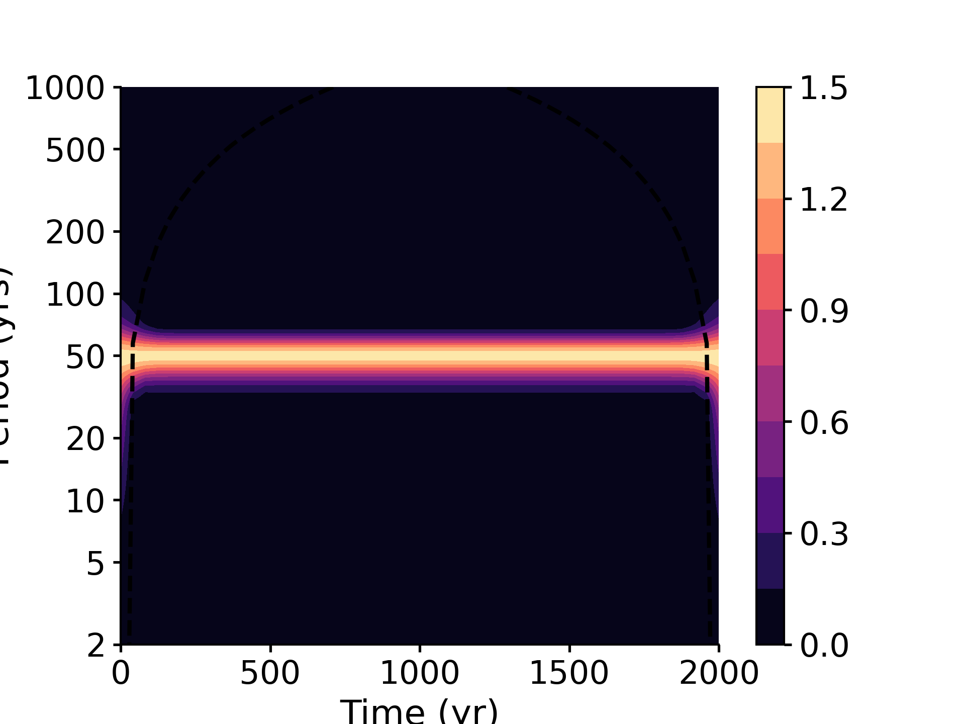
We perform an ideal test below. We use a sine wave with a period of 50 yrs as the signal for test. Then performing wavelet analysis should return an energy band around period of 50 yrs in the scalogram.

In [1]: from pyleoclim import utils

In [2]: import matplotlib.pyplot as plt

In [3]: from matplotlib.ticker import ScalarFormatter, FormatStrFormatter

In [4]: import numpy as np

# Create a signal
In [5]: time = np.arange(2001)

In [6]: f = 1/50  # the period is then 1/f = 50

In [7]: signal = np.cos(2*np.pi*f*time)

# Wavelet Analysis
In [8]: res = utils.wwz(signal, time)

# Visualization
In [9]: fig, ax = plt.subplots()

In [10]: contourf_args = {'cmap': 'magma', 'origin': 'lower', 'levels': 11}

In [11]: cbar_args = {'drawedges': False, 'orientation': 'vertical', 'fraction': 0.15, 'pad': 0.05}

In [12]: cont = ax.contourf(res.time, 1/res.freq, res.amplitude.T, **contourf_args)

In [13]: ax.plot(res.time, res.coi, 'k--')  # plot the cone of influence
Out[13]: [<matplotlib.lines.Line2D at 0x7f07d3f17040>]

In [14]: ax.set_yscale('log')

In [15]: ax.set_yticks([2, 5, 10, 20, 50, 100, 200, 500, 1000])
Out[15]: 
[<matplotlib.axis.YTick at 0x7f07e4279580>,
 <matplotlib.axis.YTick at 0x7f07d3c9cb80>,
 <matplotlib.axis.YTick at 0x7f07d3770ee0>,
 <matplotlib.axis.YTick at 0x7f07d1bf05b0>,
 <matplotlib.axis.YTick at 0x7f07d1374100>,
 <matplotlib.axis.YTick at 0x7f07d3dff7f0>,
 <matplotlib.axis.YTick at 0x7f07d3fd4280>,
 <matplotlib.axis.YTick at 0x7f07d3f3d940>,
 <matplotlib.axis.YTick at 0x7f07d3822fd0>]

In [16]: ax.set_ylim([2, 1000])
Out[16]: (2.0, 1000.0)

In [17]: ax.yaxis.set_major_formatter(ScalarFormatter())

In [18]: ax.yaxis.set_major_formatter(FormatStrFormatter('%g'))

In [19]: ax.set_xlabel('Time (yr)')
Out[19]: Text(0.5, 0, 'Time (yr)')

In [20]: ax.set_ylabel('Period (yrs)')
Out[20]: Text(0, 0.5, 'Period (yrs)')

In [21]: cb = plt.colorbar(cont, **cbar_args)

In [22]: plt.show()

pyleoclim.utils.wavelet.wwz_coherence(ys1, ts1, ys2, ts2, smooth_factor=0.25, tau=None, freq=None, freq_method='log', freq_kwargs=None, c=0.012665147955292222, Neff_threshold=3, nproc=8, detrend=False, sg_kwargs=None, verbose=False, method='Kirchner_numba', gaussianize=False, standardize=True)[source]

Returns the wavelet coherence of two time series (WWZ method).

Parameters

ys1 (array) – first of two time series
ys2 (array) – second of the two time series
ts1 (array) – time axis of first time series
ts2 (array) – time axis of the second time series
tau (array) – the evenly-spaced time points
freq (array) – vector of frequency
c (float) – the decay constant that determines the analytical resolution of frequency for analysis, the smaller the higher resolution; the default value 1/(8*np.pi**2) is good for most of the wavelet analysis cases
Neff_threshold (int) – threshold for the effective number of points
nproc (int) – the number of processes for multiprocessing
detrend (string) –
- None: the original time series is assumed to have no trend;
- ’linear’: a linear least-squares fit to ys is subtracted;
- ’constant’: the mean of ys is subtracted
- ’savitzy-golay’: ys is filtered using the Savitzky-Golay filter and the resulting filtered series is subtracted from y.
Empirical mode decomposition. The last mode is assumed to be the trend and removed from the series
sg_kwargs (dict) – The parameters for the Savitzky-Golay filter. see pyleoclim.utils.filter.savitzy_golay for details.
gaussianize (bool) – If True, gaussianizes the timeseries
standardize (bool) – If True, standardizes the timeseries
method (string) –
- ‘Foster’: the original WWZ method;
- ’Kirchner’: the method Kirchner adapted from Foster;
- ’Kirchner_f2py’: the method Kirchner adapted from Foster with f2py
- ’Kirchner_numba’: Kirchner’s algorithm with Numba support for acceleration (default)
verbose (bool) – If True, print warning messages
smooth_factor (float) – smoothing factor for the WTC (default: 0.25)

Returns

res – contains the cross wavelet coherence, cross-wavelet phase, vector of frequency, evenly-spaced time points, AR1 sims, cone of influence

Return type

dict

References

Grinsted, A., J. C. Moore, and S. Jevrejeva (2004), Application of the cross wavelet transform and wavelet coherence to geophysical time series, Nonlinear Processes in Geophysics, 11, 561–566.

See also

pyleoclim.utils.wavelet.wwz_basic: Returns the weighted wavelet amplitude using the original method from Kirchner. No multiprocessing
pyleoclim.utils.wavelet.wwz_nproc: Returns the weighted wavelet amplitude using the original method from Kirchner. Supports multiprocessing
pyleoclim.utils.wavelet.kirchner_basic: Return the weighted wavelet amplitude (WWA) modified by Kirchner. No multiprocessing
pyleoclim.utils.wavelet.kirchner_nproc: Returns the weighted wavelet amplitude (WWA) modified by Kirchner. Supports multiprocessing
pyleoclim.utils.wavelet.kirchner_numba: Return the weighted wavelet amplitude (WWA) modified by Kirchner using Numba package.
pyleoclim.utils.wavelet.kirchner_f2py: Returns the weighted wavelet amplitude (WWA) modified by Kirchner. Uses Fortran. Fastest method but requires a compiler.
pyleoclim.utils.filter.savitzky_golay: Smooth (and optionally differentiate) data with a Savitzky-Golay filter.
pyleoclim.utils.wavelet.make_freq_vector: Make frequency vector
pyleoclim.utils.tsutils.detrend: detrending functionalities
pyleoclim.utils.tsutils.gaussianize_1d: Quantile maps a 1D array to a Gaussian distribution
pyleoclim.utils.tsutils.preprocess: pre-processes a times series using Gaussianization and detrending.

Tsutils

Utilities to manipulate timeseries - useful for preprocessing prior to analysis

pyleoclim.utils.tsutils.annualize(ys, ts)[source]

Annualize a time series whose time resolution is finer than 1 year

Parameters

ys (array) – A time series, NaNs allowed
ts (array) – The time axis of the time series, NaNs allowed

Returns

ys_ann (array) – the annualized time series
year_int (array) – The time axis of the annualized time series

pyleoclim.utils.tsutils.bin(x, y, bin_size=None, start=None, stop=None, evenly_spaced=True)[source]

Bin the values

Parameters

x (array) – The x-axis series.
y (array) – The y-axis series.
bin_size (float) – The size of the bins. Default is the mean resolution if evenly_spaced is not True
start (float) – Where/when to start binning. Default is the minimum
stop (float) – When/where to stop binning. Default is the maximum
evenly_spaced ({True,False}) – Makes the series evenly-spaced. This option is ignored if bin_size is set to float

Returns

binned_values (array) – The binned values
bins (array) – The bins (centered on the median, i.e., the 100-200 bin is 150)
n (array) – Number of data points in each bin
error (array) – The standard error on the mean in each bin

See also

pyleoclim.utils.tsutils.gkernel: Coarsen time resolution using a Gaussian kernel
pyleoclim.utils.tsutils.interp: Interpolate y onto a new x-axis

pyleoclim.utils.tsutils.detrend(y, x=None, method='emd', n=1, sg_kwargs=None)[source]

Detrend a timeseries according to four methods

Detrending methods include: “linear”, “constant”, using a low-pass Savitzky-Golay filter, and Empirical Mode Decomposition (default). Linear and constant methods use [scipy.signal.detrend](https://docs.scipy.org/doc/scipy/reference/generated/scipy.signal.detrend.html), EMD uses [pyhht.emd.EMD](https://pyhht.readthedocs.io/en/stable/apiref/pyhht.html)

Parameters

y (array) – The series to be detrended.
x (array) – Abscissa for array y. Necessary for use with the Savitzky-Golay method, since the series should be evenly spaced.
method (str) – The type of detrending: - “linear”: the result of a linear least-squares fit to y is subtracted from y. - “constant”: only the mean of data is subtracted. - “savitzky-golay”, y is filtered using the Savitzky-Golay filters and the resulting filtered series is subtracted from y. - “emd” (default): Empirical mode decomposition. The last mode is assumed to be the trend and removed from the series
n (int) – Works only if method == ‘emd’. The number of smoothest modes to remove.
sg_kwargs (dict) – The parameters for the Savitzky-Golay filters.

Returns

ys – The detrended timeseries.

Return type

array

See also

pyleoclim.utils.filter.savitzky_golay: Filtering using Savitzy-Golay
pyleoclim.utils.tsutils.preprocess: pre-processes a times series using standardization and detrending.

pyleoclim.utils.tsutils.gaussianize(ys)[source]

Maps a 1D array to a Gaussian distribution using the inverse Rosenblatt transform

The resulting array is mapped to a standard normal distribution, and therefore has zero mean and unit standard deviation. Using gaussianize() obviates the need for standardize().

Parameters: ys (1D Array) – e.g. a timeseries
Returns: yg – Gaussianized values of ys.
Return type: 1D Array

References

van Albada, S., and P. Robinson (2007), Transformation of arbitrary: distributions to the normal distribution with application to EEG test-retest reliability, Journal of Neuroscience Methods, 161(2), 205 - 211, doi:10.1016/j.jneumeth.2006.11.004.

See also

pyleoclim.utils.tsutils.standardize: Centers and normalizes a time series

pyleoclim.utils.tsutils.gkernel(t, y, h=3.0, step=None, start=None, stop=None, step_style='max')[source]

Coarsen time resolution using a Gaussian kernel

Parameters

t (1d array) – the original time axis
y (1d array) – values on the original time axis
h (float) – kernel e-folding scale
step (float) –
The interpolation step. Default is max spacing between consecutive points.

start : float where/when to start the interpolation. Default is min(t).
stop (float) – where/when to stop the interpolation. Default is max(t).
step_style (str) – step style to be applied from ‘increments’ [default = ‘max’]

Returns

tc (1d array) – the coarse-grained time axis
yc (1d array) – The coarse-grained time series

References

Rehfeld, K., Marwan, N., Heitzig, J., and Kurths, J.: Comparison of correlation analysis techniques for irregularly sampled time series, Nonlin. Processes Geophys., 18, 389–404, https://doi.org/10.5194/npg-18-389-2011, 2011.

See also

pyleoclim.utils.tsutils.increments: Establishes the increments of a numerical array
pyleoclim.utils.tsutils.bin: Bin the values
pyleoclim.utils.tsutils.interp: Interpolate y onto a new x-axis

pyleoclim.utils.tsutils.interp(x, y, interp_type='linear', step=None, start=None, stop=None, step_style='mean', **kwargs)[source]

Interpolate y onto a new x-axis

Largely a wrapper for [scipy.interpolate.interp1d](https://docs.scipy.org/doc/scipy/reference/generated/scipy.interpolate.interp1d.html)

Parameters

x (array) – The x-axis
y (array) – The y-axis
interp_type (str) – Options include: ‘linear’, ‘nearest’, ‘zero’, ‘slinear’, ‘quadratic’, ‘cubic’, ‘previous’, ‘next’ where ‘zero’, ‘slinear’, ‘quadratic’ and ‘cubic’ refer to a spline interpolation of zeroth, first, second or third order; ‘previous’ and ‘next’ simply return the previous or next value of the point) or as an integer specifying the order of the spline interpolator to use. Default is ‘linear’.
step (float) – The interpolation step. Default is mean spacing between consecutive points.
start (float) – where/when to start the interpolation. Default is min..
stop (float) – where/when to stop the interpolation. Default is max.
kwargs (kwargs) – Aguments specific to interpolate.interp1D. If getting an error about extrapolation, you can use the arguments bound_errors=False and fill_value=”extrapolate” to allow for extrapolation.

Returns

xi (array) – The interpolated x-axis
yi (array) – The interpolated y values

See also

pyleoclim.utils.tsutils.increment: Establishes the increments of a numerical array
pyleoclim.utils.tsutils.bin: Bin the values
pyleoclim.utils.tsutils.gkernel: Coarsen time resolution using a Gaussian kernel

pyleoclim.utils.tsutils.remove_outliers(ts, ys, indices)[source]

Remove the outliers from timeseries data

Parameters

ts (numpy.array) – The time axis for the timeseries data.
ys (numpy.array) – The y-values for the timeseries data.
indices (numpy.array) – The indices of the outliers to be removed.

Returns

ys (numpy.array) – The time axis for the timeseries data after outliers removal
ts (numpy.array) – The y-values for the timeseries data after outliers removal

pyleoclim.utils.tsutils.simple_stats(y, axis=None)[source]

Computes simple statistics

Computes the mean, median, min, max, standard deviation, and interquartile range of a numpy array y, ignoring NaNs.

Parameters

y (array) – A Numpy array
axis (int, tuple of ints) – Axis or Axes along which the means are computed, the default is to compute the mean of the flattened array. If a tuple of ints, performed over multiple axes

Returns

mean (float) – mean of y, ignoring NaNs
median (float) – median of y, ignoring NaNs
min_ (float) – mininum value in y, ignoring NaNs
max_ (float) – max value in y, ignoring NaNs
std (float) – standard deviation of y, ignoring NaNs
IQR (float) – Interquartile range of y along specified axis, ignoring NaNs

pyleoclim.utils.tsutils.standardize(x, scale=1, axis=0, ddof=0, eps=0.001)[source]

Centers and normalizes a time series. Constant or nearly constant time series not rescaled.

Parameters

x (array) – vector of (real) numbers as a time series, NaNs allowed
scale (real) – A scale factor used to scale a record to a match a given variance
axis (int or None) – axis along which to operate, if None, compute over the whole array
ddof (int) – degress of freedom correction in the calculation of the standard deviation
eps (real) – a threshold to determine if the standard deviation is too close to zero

Returns

z (array) – The standardized time series (z-score), Z = (X - E[X])/std(X)*scale, NaNs allowed
mu (real) – The mean of the original time series, E[X]
sig (real) – The standard deviation of the original time series, std[X]

References

Tapio Schneider’s MATLAB code: https://github.com/tapios/RegEM/blob/master/standardize.m

The zscore function in SciPy: https://docs.scipy.org/doc/scipy/reference/generated/scipy.stats.zscore.html

See also

pyleoclim.utils.tsutils.preprocess: pre-processes a times series using standardization and detrending.

pyleoclim.utils.tsutils.ts2segments(ys, ts, factor=10)[source]

Chop a time series into several segments based on gap detection.

The rule of gap detection is very simple:: we define the intervals between time points as dts, then if dts[i] is larger than factor * dts[i-1], we think that the change of dts (or the gradient) is too large, and we regard it as a breaking point and chop the time series into two segments here

Parameters

ys (array) – A time series, NaNs allowed
ts (array) – The time points
factor (float) – The factor that adjusts the threshold for gap detection

Returns

seg_ys (list) – A list of several segments with potentially different lengths
seg_ts (list) – A list of the time axis of the several segments
n_segs (int) – The number of segments

Tsbase

Basic functionalities to clean timeseries data prior to analysis

pyleoclim.utils.tsbase.clean_ts(ys, ts, verbose=False)[source]

Cleaning the timeseries

Delete the NaNs in the time series and sort it with time axis ascending, duplicate timestamps will be reduced by averaging the values.

Parameters

ys (array) – A time series, NaNs allowed
ts (array) – The time axis of the time series, NaNs allowed
verbose (bool) – If True, will print a warning message

Returns

ys (array) – The time series without nans
ts (array) – The time axis of the time series without nans

See also

pyleoclim.utils.tsbase.dropna: Drop NaN values
pyleoclim.utils.tsbase.sort_ts: Sort timeseries
pyleoclim.utils.tsbase.reduce_duplicated_timestamps: Consolidate duplicated timestamps

pyleoclim.utils.tsbase.dropna(ys, ts, verbose=False)[source]

Drop NaN values

Remove entries of ys or ts that bear NaNs

Parameters

ys (array) – A time series, NaNs allowed
ts (array) – The time axis of the time series, NaNs allowed
verbose (bool) – If True, will print a warning message

Returns

ys (array) – The time series without nans
ts (array) – The time axis of the time series without nans

pyleoclim.utils.tsbase.is_evenly_spaced(ts, tol=0.0001)[source]

Check if a time axis is evenly spaced, within a given tolerance

Parameters

ts (array) – The time axis of a time series
tol (float64) – Numerical tolerance for the relative difference

Returns

check – True - evenly spaced; False - unevenly spaced.

Return type

bool

pyleoclim.utils.tsbase.reduce_duplicated_timestamps(ys, ts, verbose=False)[source]

Consolidate duplicated timestamps

Reduce duplicated timestamps in a timeseries by averaging the values

Parameters

ys (array) – Dependent variable
ts (array) – Independent variable
verbose (bool) – If True, will print a warning message

Returns

ys (array) – Dependent variable
ts (array) – Independent variable, with duplicated timestamps reduced by averaging the values

pyleoclim.utils.tsbase.sort_ts(ys, ts, verbose=False)[source]

Sort timeseries

Sort ts values in ascending order

Parameters

ys (array) – Dependent variable
ts (array) – Independent variable
verbose (bool) – If True, will print a warning message

Returns

ys (array) – Dependent variable
ts (array) – Independent variable, sorted in ascending order

Lipdutils

Utilities to manipulate LiPD files and automate data transformation whenever possible. These functions are used throughout Pyleoclim but are not meant for direct interaction by users. Also handles integration with the LinkedEarth wiki and the LinkedEarth Ontology.

jsonutils

This module converts Pyleoclim objects to and from JSON files.

Useful for obtaining a human-readable output and keeping the results of an analysis. The JSON file can also be used to swap analysis results between programming languages.

These utilities are maintained on an as-needed basis and that not all objects are currently available.

pyleoclim.utils.jsonutils.PyleoObj_to_json(obj, filename)[source]

Serializes a Pyleoclim object into a JSON file

Parameters

obj (pyleoclim.core.ui) – A Pyleoclim object from the UI module
filename (str) – Filename or path to save the JSON to.

Return type

None

See also

pyleoclim.utils.jsonutils.PyleoObj_to_dict: Encodes a Pyleoclim UI object into a dictionary that is JSON serializable

pyleoclim.utils.jsonutils.isPyleoclim(obj)[source]

Check whether an object is a valid type for Pyleoclim ui object

Parameters: obj (pyleoclim.core.ui) – Object from the Pyleoclim UI module
Returns: Bool
Return type: {True,False}

pyleoclim.utils.jsonutils.json_to_PyleoObj(filename, objname)[source]

Reads a JSON serialized file into a Pyleoclim object

Parameters

filename (str) – The filename/path/URL of the JSON-serialized object
objname (str) – Name of the object (e.g., Series, Scalogram, MultipleSeries…)

Returns

pyleoObj – A Pyleoclim UI object

Return type

pyleoclim.core.ui

See also

pyleoclim.utils.jsonutils.open_json: open a json file from a local source or URL
pyleoclim.utils.jsonutils.objename_to_obj: create a valid Pyleoclim object from a string